Main Content

Results for

I was reading Yann Debray's recent post on automating documentation with agentic AI and ended up spending more time than expected in the comments section. Not because of the comments themselves, but because of something small I noticed while trying to write one. There is no writing assistance of any kind before you post. You type, you submit, and whatever you wrote is live.
For a lot of people that is fine. But MATLAB Central has users from all over the world, and I have seen questions on MATLAB Answers where the technical reasoning is clearly correct but the phrasing makes it hard to follow. The person knew exactly what they meant. The platform just did not help them say it clearly.
I want to share a few ideas around this. They are not fully formed proposals but I think the direction is worth discussing, especially given how much AI tooling MathWorks has built recently.
What the platform has today
When you write a post in Discussions or an answer in MATLAB Answers, the editor gives you basic formatting options. Code blocks, some text styling, that is mostly it. The AI Chat Playground exists as a separate tool, and MATLAB Copilot landed in R2025a for the desktop. But none of that is inside the editor where people actually write community content.
Four things are missing that I think would make a real difference.
Grammar and clarity checking before you post
Not a forced rewrite. Just an optional Check My Draft button that highlights unclear sentences or anything that might trip a reader up. The user reviews it, decides what to change, then posts.
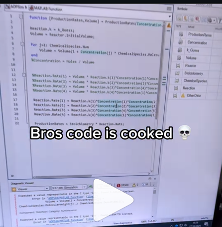
What makes this different from plugging in Grammarly is that a general-purpose tool does not know that readtable is a MATLAB function. It does not know that NaN, inf, or linspace are not errors. A MATLAB-aware checker could flag things that generic tools miss, like someone writing readTable instead of readtable in a solution post.
The llms-with-matlab package already exists on GitHub. Something like this could be built on top of it with a prompt that includes MATLAB function vocabulary as context. That is not a large lift given what is already there.
Translation support
MATLAB Central already has a Japanese-language Discussions channel. That tells you something about the community. The platform is global but most of the technical content is in English, and there is a real gap there.
Two options that would help without being intrusive:
  1. Write in your language, click Translate, review the English version, then post. The user is still responsible for what goes live.
  2. A per-post Translate button so readers can view content in a language they are more comfortable with, without changing what is stored on the platform.
A student who has the right answer to a MATLAB Answers question might not post it because they are not confident writing in English. Translation support changes that. The community gets the answer and the contributor gets the credit.
In-editor code suggestions
When someone writes a solution post they usually write the code somewhere else, test it, copy it, paste it, and format it manually. An in-editor assistant that generates a starting scaffold from a plain-text description would cut that loop down.
The key word is scaffold, not a finished answer. The label should say something like AI-generated draft, verify before posting so it is clear the person writing is still accountable. MATLAB Copilot already does something close to this inside the desktop editor. Bringing a lighter version of it into the community editor feels like a natural extension of what already exists.
A note on feasibility
These ideas are not asking for something from scratch. MathWorks already has llms-with-matlab, the MCP Core Server, and MATLAB Copilot as infrastructure. Grammar checking and translation are well-solved problems at the API level. The MATLAB-specific vocabulary awareness is the part worth investing in. None of it should be on by default. All of it should be opt-in and clearly labeled when it runs.
One more thing: diagrams in posts
Right now the only way to include a diagram in a post is to make it externally and upload an image. A lightweight drag-and-drop diagram tool inside the editor would let people show a process or structure quickly without leaving the platform. Nothing complex, just boxes and arrows. For technical explanations it is often faster to draw than to write three paragraphs.
What I am curious about
I am a Data Science student at CU Boulder and an active MATLAB user. These ideas came up while using the platform, not from a product roadmap. I do not know what is already being discussed internally at MathWorks, so it is entirely possible some of this is in progress.
Has anyone else run into the same friction points when writing on MATLAB Central? And for anyone at MathWorks who works on the community platform, is the editor something that gets investment alongside the product tools?
Happy to hear where I am wrong on the feasibility side too.
Deep Shukla || M.S. Data Science, CU Boulder || LinkedIn
AI assisted with grammar and framing. All ideas and editorial decisions are my own.
Chen Lin
Chen Lin
Last activity on 28 Jan 2026 at 20:20

A coworker shared with me a hilarious Instagram post today. A brave bro posted a short video showing his MATLAB code… casually throwing 49,000 errors!
Surprisingly, the video went virial and recieved 250,000+ likes and 800+ comments. You really never know what the Instagram algorithm is thinking, but apparently “my code is absolutely cooked” is a universal developer experience 😂
Last note: Can someone please help this Bro fix his code?
Currently, the open-source MATLAB Community is accessed via the desktop web interface, and the experience on mobile devices is not very good—especially switching between sections like Discussion, FEX, Answers, and Cody is awkward. Having a dedicated app would make using the community much more convenient on phones.
Similarty,github has Mobile APP, It's convient for me.
I struggle with animations. I often want a simple scrollable animation and wind up having to export to some external viewer in some supported format. The new Live Script automation of animations fails and sabotages other methods and it is not well documented so even AIs are clueless how to resolve issues. Often an animation works natively but not with MATLAB Online. Animation of results seems to me rather basic and should be easier!
Frequently, I find myself doing things like the following,
xyz=rand(100,3);
XYZ=num2cell(xyz,1);
scatter3(XYZ{:,1:3})
But num2cell is time-consuming, not to mention that requiring it means extra lines of code. Is there any reason not to enable this syntax,
scatter3(xyz{:,1:3})
so that I one doesn't have to go through num2cell? Here, I adopt the rule that only dimensions that are not ':' will be comma-expanded.
(Requested for newer MATLAB releases (e.g. R2026B), MATLAB Parallel Processing toolbox.)
Lower precision array types have been gaining more popularity over the years for deep learning. The current lowest precision built-in array type offered by MATLAB are 8-bit precision arrays, e.g. int8 and uint8. A good thing is that these 8-bit array types do have gpuArray support, meaning that one is able to design GPU MEX codes that take in these 8-bit arrays and reinterpret them bit-wise as other 8-bit array types, e.g. FP8, which is especially common array type used in modern day deep learning applications. I myself have used this to develop forward pass operations with 8-bit precision that are around twice as fast as 16-bit operations and with output arrays that still agree well with 16-bit outputs (measured with high cosine similarity). So the 8-bit support that MATLAB offers is already quite sufficient.
Recently, 4-bit precision array types have been shown also capable of being very useful in deep learning. These array types can be processed with Tensor Cores of more modern GPUs, such as NVIDIA's Blackwell architecture. However, MATLAB does not yet have a built-in 4-bit precision array type.
Just like MATLAB has int8 and uint8, both also with gpuArray support, it would also be nice to have MATLAB have int4 and uint4, also with gpuArray support.
Walter Roberson
Walter Roberson
Last activity on 11 Dec 2025

I can't believe someone put time into this ;-)
The formula comes from @yuruyurau. (https://x.com/yuruyurau)
digital life 1
figure('Position',[300,50,900,900], 'Color','k');
axes(gcf, 'NextPlot','add', 'Position',[0,0,1,1], 'Color','k');
axis([0, 400, 0, 400])
SHdl = scatter([], [], 2, 'filled','o','w', 'MarkerEdgeColor','none', 'MarkerFaceAlpha',.4);
t = 0;
i = 0:2e4;
x = mod(i, 100);
y = floor(i./100);
k = x./4 - 12.5;
e = y./9 + 5;
o = vecnorm([k; e])./9;
while true
t = t + pi/90;
q = x + 99 + tan(1./k) + o.*k.*(cos(e.*9)./4 + cos(y./2)).*sin(o.*4 - t);
c = o.*e./30 - t./8;
SHdl.XData = (q.*0.7.*sin(c)) + 9.*cos(y./19 + t) + 200;
SHdl.YData = 200 + (q./2.*cos(c));
drawnow
end
digital life 2
figure('Position',[300,50,900,900], 'Color','k');
axes(gcf, 'NextPlot','add', 'Position',[0,0,1,1], 'Color','k');
axis([0, 400, 0, 400])
SHdl = scatter([], [], 2, 'filled','o','w', 'MarkerEdgeColor','none', 'MarkerFaceAlpha',.4);
t = 0;
i = 0:1e4;
x = i;
y = i./235;
e = y./8 - 13;
while true
t = t + pi/240;
k = (4 + sin(y.*2 - t).*3).*cos(x./29);
d = vecnorm([k; e]);
q = 3.*sin(k.*2) + 0.3./k + sin(y./25).*k.*(9 + 4.*sin(e.*9 - d.*3 + t.*2));
SHdl.XData = q + 30.*cos(d - t) + 200;
SHdl.YData = 620 - q.*sin(d - t) - d.*39;
drawnow
end
digital life 3
figure('Position',[300,50,900,900], 'Color','k');
axes(gcf, 'NextPlot','add', 'Position',[0,0,1,1], 'Color','k');
axis([0, 400, 0, 400])
SHdl = scatter([], [], 1, 'filled','o','w', 'MarkerEdgeColor','none', 'MarkerFaceAlpha',.4);
t = 0;
i = 0:1e4;
x = mod(i, 200);
y = i./43;
k = 5.*cos(x./14).*cos(y./30);
e = y./8 - 13;
d = (k.^2 + e.^2)./59 + 4;
a = atan2(k, e);
while true
t = t + pi/20;
q = 60 - 3.*sin(a.*e) + k.*(3 + 4./d.*sin(d.^2 - t.*2));
c = d./2 + e./99 - t./18;
SHdl.XData = q.*sin(c) + 200;
SHdl.YData = (q + d.*9).*cos(c) + 200;
drawnow; pause(1e-2)
end
digital life 4
figure('Position',[300,50,900,900], 'Color','k');
axes(gcf, 'NextPlot','add', 'Position',[0,0,1,1], 'Color','k');
axis([0, 400, 0, 400])
SHdl = scatter([], [], 1, 'filled','o','w', 'MarkerEdgeColor','none', 'MarkerFaceAlpha',.4);
t = 0;
i = 0:4e4;
x = mod(i, 200);
y = i./200;
k = x./8 - 12.5;
e = y./8 - 12.5;
o = (k.^2 + e.^2)./169;
d = .5 + 5.*cos(o);
while true
t = t + pi/120;
SHdl.XData = x + d.*k.*sin(d.*2 + o + t) + e.*cos(e + t) + 100;
SHdl.YData = y./4 - o.*135 + d.*6.*cos(d.*3 + o.*9 + t) + 275;
SHdl.CData = ((d.*sin(k).*sin(t.*4 + e)).^2).'.*[1,1,1];
drawnow;
end
digital life 5
figure('Position',[300,50,900,900], 'Color','k');
axes(gcf, 'NextPlot','add', 'Position',[0,0,1,1], 'Color','k');
axis([0, 400, 0, 400])
SHdl = scatter([], [], 1, 'filled','o','w',...
'MarkerEdgeColor','none', 'MarkerFaceAlpha',.4);
t = 0;
i = 0:1e4;
x = mod(i, 200);
y = i./55;
k = 9.*cos(x./8);
e = y./8 - 12.5;
while true
t = t + pi/120;
d = (k.^2 + e.^2)./99 + sin(t)./6 + .5;
q = 99 - e.*sin(atan2(k, e).*7)./d + k.*(3 + cos(d.^2 - t).*2);
c = d./2 + e./69 - t./16;
SHdl.XData = q.*sin(c) + 200;
SHdl.YData = (q + 19.*d).*cos(c) + 200;
drawnow;
end
digital life 6
clc; clear
figure('Position',[300,50,900,900], 'Color','k');
axes(gcf, 'NextPlot','add', 'Position',[0,0,1,1], 'Color','k');
axis([0, 400, 0, 400])
SHdl = scatter([], [], 2, 'filled','o','w', 'MarkerEdgeColor','none', 'MarkerFaceAlpha',.4);
t = 0;
i = 1:1e4;
y = i./790;
k = y; idx = y < 5;
k(idx) = 6 + sin(bitxor(floor(y(idx)), 1)).*6;
k(~idx) = 4 + cos(y(~idx));
while true
t = t + pi/90;
d = sqrt((k.*cos(i + t./4)).^2 + (y/3-13).^2);
q = y.*k.*cos(i + t./4)./5.*(2 + sin(d.*2 + y - t.*4));
c = d./3 - t./2 + mod(i, 2);
SHdl.XData = q + 90.*cos(c) + 200;
SHdl.YData = 400 - (q.*sin(c) + d.*29 - 170);
drawnow; pause(1e-2)
end
digital life 7
clc; clear
figure('Position',[300,50,900,900], 'Color','k');
axes(gcf, 'NextPlot','add', 'Position',[0,0,1,1], 'Color','k');
axis([0, 400, 0, 400])
SHdl = scatter([], [], 2, 'filled','o','w', 'MarkerEdgeColor','none', 'MarkerFaceAlpha',.4);
t = 0;
i = 1:1e4;
y = i./345;
x = y; idx = y < 11;
x(idx) = 6 + sin(bitxor(floor(x(idx)), 8))*6;
x(~idx) = x(~idx)./5 + cos(x(~idx)./2);
e = y./7 - 13;
while true
t = t + pi/120;
k = x.*cos(i - t./4);
d = sqrt(k.^2 + e.^2) + sin(e./4 + t)./2;
q = y.*k./d.*(3 + sin(d.*2 + y./2 - t.*4));
c = d./2 + 1 - t./2;
SHdl.XData = q + 60.*cos(c) + 200;
SHdl.YData = 400 - (q.*sin(c) + d.*29 - 170);
drawnow; pause(5e-3)
end
digital life 8
clc; clear
figure('Position',[300,50,900,900], 'Color','k');
axes(gcf, 'NextPlot','add', 'Position',[0,0,1,1], 'Color','k');
axis([0, 400, 0, 400])
SHdl{6} = [];
for j = 1:6
SHdl{j} = scatter([], [], 2, 'filled','o','w', 'MarkerEdgeColor','none', 'MarkerFaceAlpha',.3);
end
t = 0;
i = 1:2e4;
k = mod(i, 25) - 12;
e = i./800; m = 200;
theta = pi/3;
R = [cos(theta) -sin(theta); sin(theta) cos(theta)];
while true
t = t + pi/240;
d = 7.*cos(sqrt(k.^2 + e.^2)./3 + t./2);
XY = [k.*4 + d.*k.*sin(d + e./9 + t);
e.*2 - d.*9 - d.*9.*cos(d + t)];
for j = 1:6
XY = R*XY;
SHdl{j}.XData = XY(1,:) + m;
SHdl{j}.YData = XY(2,:) + m;
end
drawnow;
end
digital life 9
clc; clear
figure('Position',[300,50,900,900], 'Color','k');
axes(gcf, 'NextPlot','add', 'Position',[0,0,1,1], 'Color','k');
axis([0, 400, 0, 400])
SHdl{14} = [];
for j = 1:14
SHdl{j} = scatter([], [], 2, 'filled','o','w', 'MarkerEdgeColor','none', 'MarkerFaceAlpha',.1);
end
t = 0;
i = 1:2e4;
k = mod(i, 50) - 25;
e = i./1100; m = 200;
theta = pi/7;
R = [cos(theta) -sin(theta); sin(theta) cos(theta)];
while true
t = t + pi/240;
d = 5.*cos(sqrt(k.^2 + e.^2) - t + mod(i, 2));
XY = [k + k.*d./6.*sin(d + e./3 + t);
90 + e.*d - e./d.*2.*cos(d + t)];
for j = 1:14
XY = R*XY;
SHdl{j}.XData = XY(1,:) + m;
SHdl{j}.YData = XY(2,:) + m;
end
drawnow;
end
Ludvig Nordin
Ludvig Nordin
Last activity on 13 Nov 2025

Pure Matlab
82%
Simulink
18%
11 votes
Jorge Bernal-AlvizJorge Bernal-Alviz shared the following code that requires R2025a or later:
Test()
Warning: Hardware-accelerated graphics is unavailable. Displaying fewer markers to preserve interactivity.
function Test()
duration = 10;
numFrames = 800;
frameInterval = duration / numFrames;
w = 400;
t = 0;
i_vals = 1:10000;
x_vals = i_vals;
y_vals = i_vals / 235;
r = linspace(0, 1, 300)';
g = linspace(0, 0.1, 300)';
b = linspace(1, 0, 300)';
r = r * 0.8 + 0.1;
g = g * 0.6 + 0.1;
b = b * 0.9 + 0.1;
customColormap = [r, g, b];
figure('Position', [100, 100, w, w], 'Color', [0, 0, 0]);
axis equal;
axis off;
xlim([0, w]);
ylim([0, w]);
hold on;
colormap default;
colormap(customColormap);
plothandle = scatter([], [], 1, 'filled', 'MarkerFaceAlpha', 0.12);
for i = 1:numFrames
t = t + pi/240;
k = (4 + 3 * sin(y_vals * 2 - t)) .* cos(x_vals / 29);
e = y_vals / 8 - 13;
d = sqrt(k.^2 + e.^2);
c = d - t;
q = 3 * sin(2 * k) + 0.3 ./ (k + 1e-10) + ...
sin(y_vals / 25) .* k .* (9 + 4 * sin(9 * e - 3 * d + 2 * t));
points_x = q + 30 * cos(c) + 200;
points_y = q .* sin(c) + 39 * d - 220;
points_y = w - points_y;
CData = (1 + sin(0.1 * (d - t))) / 3;
CData = max(0, min(1, CData));
set(plothandle, 'XData', points_x, 'YData', points_y, 'CData', CData);
brightness = 0.5 + 0.3 * sin(t * 0.2);
set(plothandle, 'MarkerFaceAlpha', brightness);
drawnow;
pause(frameInterval);
end
end
From my experience, MATLAB's Deep Learning Toolbox is quite user-friendly, but it still falls short of libraries like PyTorch in many respects. Most users tend to choose PyTorch because of its flexibility, efficiency, and rich support for many mathematical operators. In recent years, the number of dlarray-compatible mathematical functions added to the toolbox has been very limited, which makes it difficult to experiment with many custom networks. For example, svd is currently not supported for dlarray inputs.
This link (List of Functions with dlarray Support - MATLAB & Simulink) lists all functions that support dlarray as of R2026a — only around 200 functions (including toolbox-specific ones). I would like to see support for many more fundamental mathematical functions so that users have greater freedom when building and researching custom models. For context, the core MATLAB mathematics module contains roughly 600 functions, and many application domains build on that foundation.
I hope MathWorks will prioritize and accelerate expanding dlarray support for basic math functions. Doing so would significantly increase the Deep Learning Toolbox's utility and appeal for researchers and practitioners.
Thank you.
I'm working on training neural networks without backpropagation / automatic differentiation, using locally derived analytic forms of update rules. Given that this allows a direct formula to be derived for the update rule, it removes alot of the overhead that is otherwise required from automatic differentiation.
However, matlab's functionalities for neural networks are currently solely based around backpropagation and automatic differentiation, such as the dlgradient function and requiring everything to be dlarrays during training.
I have two main requests, specifically for functions that perform a single operation within a single layer of a neural network, such as "dlconv", "fullyconnect", "maxpool", "avgpool", "relu", etc:
  • these functions should also allow normal gpuArray data instead of requiring everything to be dlarrays.
  • these functions are currently designed to only perform the forward pass. I request that these also be designed to perform the backward pass if user requests. There can be another input user flag that can be "forward" (default) or "backward", and then the function should have all the necessary inputs to perform that operation (e.g. for "avgpool" forward pass it only needs the avgpool input data and the avgpool parameters, but for the "avgpool" backward pass it needs the deriviative w.r.t. the avgpool output data, the avgpool parameters, and the original data dimensions). I know that there is a maxunpool function that achieves this for maxpool, but it has significant issues when trying to use it this way instead of by backpropagation in a dlgradient type layer, see (https://www.mathworks.com/matlabcentral/answers/2179587-making-a-custom-way-to-train-cnns-and-i-am-noticing-that-avgpool-is-significantly-faster-than-maxpo?s_tid=srchtitle).
I don't know how many people would benefit from this feature, and someone could always spend their time creating these functionalities themselves by matlab scripts, cuDNN mex, etc., but regardless it would be nice for matlab to have this allowable for more customizable neural net training.
Inspired by @xingxingcui's post about old MATLAB versions and @유장's post about an old Easter egg, I thought it might be fun to share some MATLAB-Old-Timer Stories™.
Back in the early 90s, MATLAB had been ported to MacOS, but there were some interesting wrinkles. One that kept me earning my money as a computer lab tutor was that MATLAB required file names to follow Windows standards - no spaces or other special characters. But on a Mac, nothing stopped you from naming your script "hello world - 123.m". The problem came when you tried to run it. MATLAB was essentially doing an eval on the script name, assuming the file name would follow Windows (and MATLAB) naming rules.
So now imagine a lab full of students taking a university course. As is common in many universities, the course was given a numeric code. For whatever historical reason, my school at that time was also using numeric codes for the departments. Despite being told the rules for naming scripts, many students would default to something like "26.165 - 1.1" for problem one on HW1 for the intro applied math course 26.165.
No matter what they did in their script, when they ran it, MATLAB would just say "ans = 25.0650".
Nothing brings you more MATLAB-god credibility as a student tutor than walking over to someone's computer, taking one look at their output, saying "rename your file", and walking away like a boss.
It was 2010 when I was a sophomore in university. I chose to learn MATLAB because of a mathematical modeling competition, and the university provided MATLAB 7.0, a very classic release. To get started, I borrowed many MATLAB books from the library and began by learning simple numerical calculations, plotting, and solving equations. Gradually I was drawn in by MATLAB’s powerful capabilities and became interested; I often used it as a big calculator for fun. That version didn’t have MATLAB Live Script; instead it used MATLAB Notebook (M-Book), which allowed MATLAB functions to be used directly within Microsoft Word, and it also had the Symbolic Math Toolbox’s MuPAD interactive environment. These were later gradually replaced by Live Scripts introduced in R2016a. There are many similar examples...
Out of curiosity, I still have screenshots on my computer showing MATLAB 7.0 running compatibly. I’d love to hear your thoughts?
Edit 15 Oct 2025: Removed incorrect code. Replaced symmatrix2sym and symfunmatrix2symfun with sym and symfun respectively (latter supported as of 2024b).
The Symbolic Math Toolbox does not have its own dot and and cross functions. That's o.k. (maybe) for garden variety vectors of sym objects where those operations get shipped off to the base Matlab functions
x = sym('x',[3,1]); y = sym('y',[3,1]);
which dot(x,y)
/MATLAB/toolbox/matlab/specfun/dot.m
dot(x,y)
ans = 
which cross(x,y)
/MATLAB/toolbox/matlab/specfun/cross.m
cross(x,y)
ans = 
But now we have symmatrix et. al., and things don't work as nicely
clearvars
x = symmatrix('x',[3,1]); y = symmatrix('y',[3,1]);
z = symmatrix('z',[1,1]);
sympref('AbbreviateOutput',false);
dot() expands the result, which isn't really desirable for exposition.
eqn = z == dot(x,y)
eqn = 
Also, dot() returns the the result in terms of the conjugate of x, which can't be simplifed away at the symmatrix level
assumeAlso(sym(x),'real')
class(eqn)
ans = 'symmatrix'
try
eqn = z == simplify(dot(x,y))
catch ME
ME.message
end
ans = 'Undefined function 'simplify' for input arguments of type 'symmatrix'.'
To get rid of the conjugate, we have to resort to sym
eqn = simplify(sym(eqn))
eqn = 
but again we are in expanded form, which defeats the purpose of symmatrix (et. al.)
But at least we can do this to get a nice equation
eqn = z == x.'*y
eqn = 
dot errors with symfunmatrix inputs
clearvars
syms t real
x = symfunmatrix('x(t)',t,[3,1]); y = symfunmatrix('y(t)',t,[3,1]);
try
dot(x,y)
catch ME
ME.message
end
ans = 'Invalid argument at position 2. Symbolic function is evaluated at the input arguments and does not accept colon indexing. Instead, use FORMULA on the function and perform colon indexing on the returned output.'
Cross works (accidentally IMO) with symmatrix, but expands the result, which isn't really desirable for exposition
clearvars
x = symmatrix('x',[3,1]); y = symmatrix('y',[3,1]);
z = symmatrix('z',[3,1]);
eqn = z == cross(x,y)
eqn = 
And it doesn't work at all if an input is a symfunmatrix
syms t
w = symfunmatrix('w(t)',t,[3,1]);
try
eqn = z == cross(x,w);
catch ME
ME.message
end
ans = 'A and B must be of length 3 in the dimension in which the cross product is taken.'
In the latter case we can expand with
eqn = z == cross(sym(x),symfun(w)) % x has to be converted
eqn(t) = 
But we can't do the same with dot (as shown above, dot doesn't like symfun inputs)
try
eqn = z == dot(sym(x),symfun(w))
catch ME
ME.message
end
ans = 'Invalid argument at position 2. Symbolic function is evaluated at the input arguments and does not accept colon indexing. Instead, use FORMULA on the function and perform colon indexing on the returned output.'
Looks like the only choice for dot with symfunmatrix is to write it by hand at the matrix level
x.'*w
ans(t) = 
or at the sym/symfun level
sym(x).'*symfun(w) % assuming x is real
ans(t) = 
Ideally, I'd like to see dot and cross implemented for symmatrix and symfunmatrix types where neither function would evaluate, i.e., expand, until both arguments are subs-ed with sym or symfun objects of appropriate dimension.
Also, it would be nice if symmatrix could be assumed to be real. Is there a reason why being able to do so wouldn't make sense?
try
assume(x,'real')
catch ME
ME.message
end
ans = 'Undefined function 'assume' for input arguments of type 'symmatrix'.'
Automating Parameter Identifiability Analysis in SimBiology
Is it possible to develop a MATLAB Live Script that automates a series of SimBiology model fits to obtain likelihood profiles? The goal is to fit a kinetic model to experimental data while systematically fixing the value of one kinetic constant (e.g., k1) and leaving the others unrestricted.
The script would perform the following:
Use a pre-configured SimBiology project where the best fit to the experimental data has already been established (including dependent/independent variables, covariates, the error model, and optimization settings).
Iterate over a defined sequence of fixed values for a chosen parameter.
For each fixed value, run the estimation to optimize the remaining parameters.
Record the resulting Sum of Squared Errors (SSE) for each run.
The final output would be a likelihood profile—a plot of SSE versus the fixed parameter value (e.g., k1)—to assess the practical identifiability of each model parameter.
Something that I periodically wonder about is whether an integration with the Rubi integration rules package would improve symbolic integration in Matlab's Symbolic Toolbox. The project is open-source with an MIT-licensed, has a Mathematica implementation, and supposedly SymPy is working on an implementation. Much of my intrigue comes from this 2022 report that compared the previous version of Rubi (4.16.1) against various CAS systems, including Matlab 2021a (Mupad):
While not really an official metric for Rubi, this does "feel" similar to my experience computing symbolic integrals in Matlab Symbolic Toolbox vs Maple/Mathematica. What do y'all think?
Have you ever been enrolled in a course that uses an LMS and there is an assignment that invovles posting a question to, or answering a question in, a discussion group? This discussion group is meant to simulate that experience.