Results for
The "Issues" with Constant Properties
MATLABs Constant properties can be rather difficult to deal with at times. For those unfamiliar there are two distinct behaviors when accessing constant properties of a class. If a "static" pattern is used ClassName.PropName the the value, as it was assigned to the property is returned; that is to say that you will have a nargout of 1. But, rather frustratingly, if an instance of the class is used when accessing the constant property, such as ArrayOfClassName.PropName then your nargout will be equivalent to the number of elements in the array; this means that functionally the constant property accessing scheme is identical to that of the element wise properties you find on "instance" properties.
Motivation for Correcting Constant Property Behavior
This can be frustraing since constant properties are conceptually designed to tie data to a class. You could see this design pattern being useful where a super class were to define an abstract constant property, that would drive the behavior of subclasses; the subclasses define the value of the property and the super class uses it. I would like to use this design to develop a custom display "MatrixDisplay" focused mixin (like the internal matlab.mixin.internal.MatrixDisplay). The idea is that missing element labels, invalid handle element labels, and other semantic values can be configured by the subclasses, conveniently just by setting the constant properties; these properties will be used by the super class to substitute the display strings of appropriate elements. Most of the processing will happen within the super class as to enable simple, low-investment, opt-in display options for array style classes.
The issue is that you can not rely on constant property access to return the appropriate value when the instance you've been passed is empty. This also happens with excessive outputs when the instance is non-scalar, but those extra values from the CSL are just ignored, while Id imagine there is an effect on performance from generating the excess outputs (assuming theres no internal optimization for the unused outputs), this case still functions appropriately. As I enjoying exploring MATLAB, I found an internal indexing mixing class in the past that provides far greater control of do indexing; I've done a good deal of neat things with it, though at the cost of great overhead when getting implementing cool "proof of concept/showcase" examples. Today I used it to quickly implement a mix in that "fixes" constant properties such that they always return as though they were called statically from the class name, as opposed to an instance.
A Simplistic Solution
To do this I just intercepted the property indexing, checked if it was constant, and used the DefaultValue property of the metadata to return the value. This works nicely since we are required to attempt to initialize a "dummy" scalar array, or generate a function handle; both of those would likely be slower, and in the former case, may not be possible depending on the subclass implementation. It is worth noting that this method of querying the value from metadata is safe because constant properties are immutable and thus must be established as the class is loaded. Below is the small utility class I have implemented to get predictable constant variable access into classes that benefit from it. Lastly it is worth noting that I've not torture testing the rerouting of the indexing we aren't intercepting, in my limited play its behaved as expected but it may be worth looking over if you end up playing around with this and notice abnormal property assignment or reading from non-constant properties.
Sample Class Implementation
classdef(Abstract, HandleCompatible) ConstantProperty < matlab.mixin.internal.indexing.RedefinesDotProperties
%ConstantProperty Returns instance indexed constant properties as though they were statically indexed.
% This class overloads property access to check if the indexed property is constant and return it properly.
%% Property membership utility methods
methods(Access=private)
function [isConst, isProp] = isConstantProp(obj, prop, options)
%isConstantProp Determine if the input property names are constant properties of the input
arguments
obj mixin.ConstantProperty;
prop string;
options.Flatten (1, 1) logical = false;
end
% Store the cache to avoid rechecking string membership and parsing metadata
persistent class_cache
% Initialize cache for all subclasses to maintain their own caches
if(isempty(class_cache))
class_cache = configureDictionary("string", "dictionary");
end
% Gather the current class being analyzed
classname = string(class(obj));
% Check if the current class has a cache, if not make one
if(~isKey(class_cache, classname))
class_cache(classname) = configureDictionary("string", "struct");
end
% Alias the current classes cache
prop_cache = class_cache(classname);
% Check which inputs are already cached
isCached = isKey(prop_cache, prop);
% Add any values that have yet to be cached to the cache
if(any(~isCached, "all"))
% Flatten cache additions
props = row(prop(~isCached));
% Gather the meta-property data of the input object and determine if inputs are listed properties
mc_props = metaclass(obj).PropertyList;
% Determine which properties are keys
[isConst, idx] = ismember(props, string({mc_props.Name}));
idx = idx(isConst);
% Check which of the inputs are constant properties
isConst = repmat(isConst, 2, 1);
isConst(1, isConst(1, :)) = [mc_props(idx).Constant];
% Parse the results into structs for caching
cache_values = cell2struct(num2cell(isConst), ["isConst"; "isProp"]);
prop_cache(props) = row(cache_values);
% Re-sync the cache
class_cache(classname) = prop_cache;
end
% Extract results from the cache
values = prop_cache(prop);
if(options.Flatten)
% Split and reshape output data
sz = size(prop);
isConst = reshape(values.isConst, sz);
isProp = reshape(values.isProp, sz);
else
isConst = struct2cell(values);
end
end
function [isConst, isProp] = isConstantIdxOp(obj, idxOp)
%isConstantIdxOp Determines if the idxOp is referencing a constant property.
arguments
obj mixin.ConstantProperty;
idxOp (1, :) matlab.indexing.IndexingOperation;
end
import matlab.indexing.IndexingOperationType;
if(idxOp(1).Type == IndexingOperationType.Dot)
[isConst, isProp] = isConstantProp(obj, idxOp(1).Name);
else
[isConst, isProp] = deal(false);
end
end
function A = getConstantProperty(obj, idxOp)
%getConstantProperty Returns the value of a constant property using a static reference pattern.
arguments
obj mixin.ConstantProperty;
idxOp (1, :) matlab.indexing.IndexingOperation;
end
A = findobj(metaclass(obj).PropertyList, "Name", idxOp(1).Name).DefaultValue;
end
end
%% Dot indexing methods
methods(Access = protected)
function A = dotReference(obj, idxOp)
arguments(Input)
obj mixin.ConstantProperty;
idxOp (1, :) matlab.indexing.IndexingOperation;
end
arguments(Output, Repeating)
A
end
% Force at least one output
N = max(1, nargout);
% Check if the indexing operation is a property, and if that property is constant
[isConst, isProp] = isConstantIdxOp(obj, idxOp);
if(~isProp)
% Error on invalid properties
throw(MException( ...
"JB:mixin:ConstantProperty:UnrecognizedProperty", ...
"Unrecognized property '%s'.", ...
idxOp(1).Name ...
));
elseif(isConst)
% Handle forwarding indexing operations
if(isscalar(idxOp))
% Direct assignment
[A{1:N}] = getConstantProperty(obj, idxOp);
else
% First extract constant property then forward indexing operations
tmp = getConstantProperty(obj, idxOp);
[A{1:N}] = tmp.(idxOp(2:end));
end
else
% Handle forwarding indexing operations
if(isscalar(idxOp))
% Unfortunately we can't just recall obj.(idxOp) to use default/built-in so we manually extract
[A{1:N}] = obj.(idxOp.Name);
else
% Otherwise let built-in handling proceed
tmp = obj.(idxOp(1).Name);
[A{1:N}] = tmp.(idxOp(2:end));
end
end
end
function obj = dotAssign(obj, idxOp, values)
arguments(Input)
obj mixin.ConstantProperty;
idxOp (1, :) matlab.indexing.IndexingOperation;
end
arguments(Input, Repeating)
values
end
% Handle assignment based on presence of forward indexing
if(isscalar(idxOp))
% Simple broadcasted assignment
[obj.(idxOp.Name)] = deal(values{:});
else
% Initialize the intermediate values and expand the values for assignment
tmp = {obj.(idxOp(1).Name)};
[tmp.(idxOp(2:end))] = deal(values{:});
% Reassign the modified data to the output object
[obj.(idxOp(1).Name)] = deal(tmp{:});
end
end
function n = dotListLength(obj, idxOp, idxCnt)
arguments(Input)
obj mixin.ConstantProperty;
idxOp (1, :) matlab.indexing.IndexingOperation;
idxCnt (1, :) matlab.indexing.IndexingContext;
end
if(isConstantIdxOp(obj, idxOp))
if(isscalar(idxOp))
% Constant properties will also be 1
n = 1;
else
% Checking forwarded indexing operations on the scalar constant property
n = listLength(obj.(idxOp(1).Name), idxOp(2:end), idxCnt);
end
else
% Check the indexing operation normally
% n = listLength(obj, idxOp, idxCnt);
n = numel(obj);
end
end
end
end
k-Wave is a MATLAB community toolbox with a track record that includes over 2,500 citations on Google Scholar and over 7,500 downloads on File Exchange. It is built for the "time-domain simulation of acoustic wave fields" and was recently highlighted as a Pick of the Week.
In December, release v1.4.1 was published on GitHub including two new features led by the project's core contributors with domain experts in this field. This first release in several years also included quality and maintainability enhancements supported by a new code contributor, GitHub user stellaprins, who is a Research Software Engineer at University College London. Her contributions in 2025 spanned several software engineering aspects, including the addition of continuous integration (CI), fixing several bugs, and updating date/time handling to use datetime. The MATLAB Community Toolbox Program sponsored these contributions, and welcomes to see them now integrated into a release for k-Wave users.
I'd like to share some work from Controls Educator and long term collabortor @Dr James E. Pickering from Harper Adams University. He is currently developing a teaching architecture for control engineering (ACE-CORE) and is looking for feedback from the engineering community.
ACE-CORE is delivered through ACE-Box, a modular hardware platform (Base + Sense, Actuate). More on the hardware here: What is the ACE-Box?
The Structure
(1) Comprehend
Learners build conceptual understanding of control systems by mapping block diagrams directly to physical components and signals. The emphasis is on:
- Feedback architecture
- Sensing and actuation
- Closed-loop behaviour in practical terms
(2) Operate
Using ACE-Box (initially Base + Sense), learners run real closed-loop systems. The learners measure, actuate, and observe real phenomena such as: Noise, Delay, Saturation
Engineering requirements (settling time, overshoot, steady-state error, etc.) are introduced explicitly at this stage.
After completing core activities (e.g., low-pass filter implementation or PID tuning), the pathway branches (see the attached diagram)
(3a) Refine (Option 1) Students improve performance through structured tuning:
- PID gains
- Filter coefficients
- Performance trade-offs
The focus is optimisation against defined engineering requirements.
(3b) Refine → Engineer (Option 2)
Modelling and analytical design become more explicit at this stage, including:
- Mathematical modelling
- Transfer functions
- System identification
- Stability analysis
- Analytical controller design
Why the Branching?
The structure reflects two realities:
- Engineers who operate and refine existing control systems
- Engineers who design control systems through mathematical modelling
Your perspective would be very valuable:
- Does this progression reflect industry reality?
- Is the branching structure meaningful?
- What blind spots do you see?
Constructive critique is very welcome. Thank you!
I coded this app to solve the 20 or so test cases included with the Cody problem 'visually' and step-by-step. For extra fun, it can also be used to play the game... Any comments or suggestions welcome!
I wanted to share something I've been thinking about to get your reactions. We all know that most MATLAB users are engineers and scientists, using MATLAB to do engineering and science. Of course, some users are professional software developers who build professional software with MATLAB - either MATLAB-based tools for engineers and scientists, or production software with MATLAB Coder, MATLAB Compiler, or MATLAB Web App Server.
I've spent years puzzling about the very large grey area in between - engineers and scientists who build useful-enough stuff in MATLAB that they want their code to work tomorrow, on somebody else's machine, or maybe for a large number of users. My colleagues and I have taken to calling them "Reluctant Developers". I say "them", but I am 1,000% a reluctant developer.
I first hit this problem while working on my Mech Eng Ph.D. in the late 90s. I built some elaborate MATLAB-based tools to run experiments and analysis in our lab. Several of us relied on them day in and day out. I don't think I was out in the real world for more than a month before my advisor pinged me because my software stopped working. And so began a career of building amazing, useful, and wildly unreliable tools for other MATLAB users.
About a decade ago I noticed that people kept trying to nudge me along - "you should really write tests", "why aren't you using source control". I ignored them. These are things software developers do, and I'm an engineer.
I think it finally clicked for me when I listened to a talk at a MATLAB Expo around 2017. An aerospace engineer gave a talk on how his team had adopted git-based workflows for developing flight control algorithms. An attendee asked "how do you have time to do engineering with all this extra time spent using software development tools like git"? The response was something to the effect of "oh, we actually have more time to do engineering. We've eliminated all of the waste from our unamanaged processes, like multiple people making similar updates or losing track of the best version of an algorithm." I still didn't adopt better practices, but at least I started to get a sense of why I might.
Fast-forward to today. I know lots of users who've picked up software dev tools like they are no big deal, but I know lots more who are still holding onto their ad-hoc workflows as long as they can. I'm on a bit of a campaign to try to change this. I'd like to help MATLAB users recognize when they have problems that are best solved by borrowing tools from our software developer friends, and then give a gentle onramp to using these tools with MATLAB.
I recently published this guide as a start:
Waddya think? Does the idea of Reluctant Developer resonate with you? If you take some time to read the guide, I'd love comments here or give suggestions by creating Issues on the guide on GitHub (there I go, sneaking in some software dev stuff ...)
DocMaker allows you to create MATLAB toolbox documentation from Markdown documents and MATLAB scripts.
The MathWorks Consulting group have been using it for a while now, and so David Sampson, the director of Application Engineering, felt that it was time to share it with the MATLAB and Simulink community.
David listed its features as:
➡️ write documentation in Markdown not HTML
🏃 run MATLAB code and insert textual and graphical output
📜 no more hand writing XML index files
🕸️ generate documentation for any release from R2021a onwards
💻 view and edit documentation in MATLAB, VS Code, GitHub, GitLab, ...
🎉 automate toolbox documentation generation using MATLAB build tool
📃 fully documented using itself
😎 supports light, dark, and responsive modes
🐣 cute logo
I got an email message that says all the files I've uploaded to the File Exchange will be given unique names. Are these new names being applied to my files automatically? If so, do I need to download them to get versions with the new name so that if I update them they'll have the new name instead of the name I'm using now?
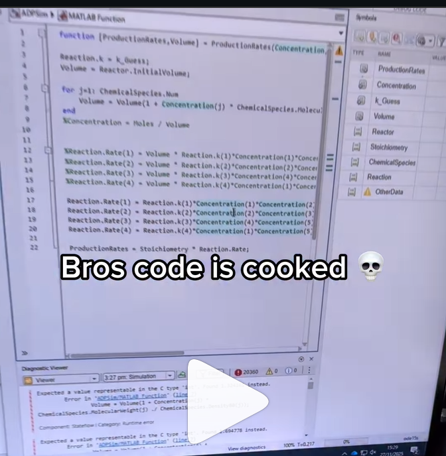
A coworker shared with me a hilarious Instagram post today. A brave bro posted a short video showing his MATLAB code… casually throwing 49,000 errors!
Surprisingly, the video went virial and recieved 250,000+ likes and 800+ comments. You really never know what the Instagram algorithm is thinking, but apparently “my code is absolutely cooked” is a universal developer experience 😂
Last note: Can someone please help this Bro fix his code?
In 2025, we saw the growing impact of GenAI on site traffic and user behavior across the entire technical landscape. Amid all this change, MATLAB Central continued to stand out as a trusted home for MATLAB and Simulink users. More than 11 million unique visitors in 2025 came to MATLAB Central to ask questions, share code, learn, and connect with one another.
Let’s celebrate what made 2025 memorable across three key areas: people, content, and events.
People
In 2025, nearly 20,000 contributors participated across the community. We’d like to spotlight a few standout contributors:
- @Sam Chak earned the Most Accepted Answers Badge for both 2024 and 2025. Sam is a rising star in MATLAB Answers with 2,000+ answers and 1,000+ votes.
- @Rodney Tan has been actively contributing files to File Exchange. In 2025, his submissions got almost 20,000 downloads!
- @Dyuman Joshi was recognized as a top contributor on both Cody and Answers. Many may not know that Dyuman is also a Cody moderator, doing tremendous behind-the-scenes moderation work to keep the platform running smoothly.
- A warm welcome to @Steve Eddins, who joined the Community Advisory Board. Steve brings a unique perspective as a former MathWorker and long-time top community contributor.
- Congratulations to @Walter Roberson on reaching 100 followers! MATLAB Central thrives on people-to-people connections, and we’d love to see even more of these relationships grow.
Of course, there are many contributors we didn’t mention here—thank you all for your outstanding contributions and for making the community what it is.
Content
Our high-quality community content not only attracts users but also helps power the broader GenAI ecosystem.
Popular Blog Post & File Exchange Submission
- Zoomed Axes, submitted by @Caleb Thomas, enables zoomed-in views of selected regions in a plot.This submission was featured in the Pick of the Week blog post, “MATLAB Zoomed Axes: Showing zoomed-in regions of a 2D plot,” which generated 5,000 views in just one month.
Popular Discussion Post
- What did MATLAB/Simulink users wait for most in 2025? It's R2025a! “Where is MATLAB R2025a?” became the most-viewed discussion post, with 10,000 views and 30 comments. Thanks for your patience — MATLAB R2025a turned out to be one of the biggest releases we’ve ever delivered.
Most Viewed Question
- “How do I create a for loop in MATLAB?” was the most-viewed community question of the year. It’s a fun reminder that even as MATLAB evolves, the basics remain essential — and always in demand.
Most Voted Poll
- “Did you know there is an official MATLAB certification?”, created by @goc3, was the most-voted poll of 2025.While 50% of respondents voted “No”, it’s exciting to see 3% are certified MATLAB Professionals. Will you be one of them in 2026?
Events
The Cody Contest 2025 brought teams together to tackle challenging but fun Cody problems. During the contest:
- 20,000+ solutions were submitted
- 20+ tips & tricks articles were shared by top players
While the contest has ended, you can still challenge yourself with the fun contest problem group. If you get stuck, the tips & tricks articles are a great resource—and you’ll be amazed by the creativity and skill of the contributors.
Thank you for being part of an incredible 2025. Your curiosity, generosity, and expertise are what make MATLAB Central a trusted home for millions—and we look forward to learning and growing together in 2026.
https://www.mathworks.com/matlabcentral/answers/2182045-why-can-t-i-renew-or-purchase-add-ons-for-m…
"As of January 1, 2026, Perpetual Student and Home offerings have been sunset and replaced with new Annual Subscription Student and Home offerings."
So, Perpetual licenses for Student and Home versions are no more. Also, the ability for Student and Home to license just MATLAB by itself has been removed.
The new offering for Students is $US119 per year with no possibility of renewing through a Software Maintenance Service type offering. That $US119 covers the Student Suite of MATLAB and Simulink and 11 other toolboxes. Before, the perpetual license was $US99... and was a perpetual license, so if (for example) you bought it in second year you could use it in third and fourth year for no additional cost. $US99 once, or $US99 + $US35*2 = $US169 (if you took SMS for 2 years) has now been replaced by $US119 * 3 = $US357 (assuming 3 years use.)
The new offering for Home is $US165 per year for the Suite (MATLAB + 12 common toolboxes.) This is a less expensive than the previous $US150 + $US49 per toolbox if you had a use for those toolboxes . Except the previous price was a perpetual license. It seems to me to be more likely that Home users would have a use for the license for extended periods, compared to the Student license (Student licenses were perpetual licenses but were only valid while you were enrolled in degree granting instituations.)
Unfortunately, I do not presently recall the (former) price for SMS for the Home license. It might be the case that by the time you added up SMS for base MATLAB and the 12 toolboxes, that you were pretty much approaching $US165 per year anyhow... if you needed those toolboxes and were willing to pay for SMS.
But any way you look at it, the price for the Student version has effectively gone way up. I think this is a bad move, that will discourage students from purchasing MATLAB in any given year, unless they need it for courses. No (well, not much) more students buying MATLAB with the intent to explore it, knowing that it would still be available to them when it came time for their courses.
In the sequence of previous suggestion in Meta Cody comment for the 'My Problems' page, I also suggest to add a red alert for new comments in 'My Groups' page.
Thank you in advance.
Give your LLM an easier time looking for information on mathworks.com: point it to the recently released llms.txt files. The top-level one is www.mathworks.com/llms.txt, release changes use www.mathworks.com/help/relnotes. How does it work for you??
I can't believe someone put time into this ;-)

Our exportgraphics and copygraphics functions now offer direct and intuitive control over the size, padding, and aspect ratio of your exported figures.
- Specify Output Size: Use the new Width, Height, and Units name-value pairs
- Control Padding: Easily adjust the space around your axes using the Padding argument, or set it to to match the onscreen appearance.
- Preserve Aspect Ratio: Use PreserveAspectRatio='on' to maintain the original plot proportions when specifying a fixed size.
- SVG Export: The exportgraphics function now supports exporting to the SVG file format.
Check out the full article on the Graphics and App Building blog for examples and details: Advanced Control of Size and Layout of Exported Graphics
No, staying home (or where I'm now)
25%
Yes, 1 night
0%
Yes, 2 nights
12.5%
Yes, 3 nights
12.5%
Yes, 4-7 nights
25%
Yes, 8 nights or more
25%
8 votes
I believe that it is very useful and important to know when we have new comments of our own problems. Although I had chosen to receive notifications about my own problems, I only receive them when I am mentioned by @.
Is it possible to add a 'New comment' alert in front of each problem on the 'My Problems' page?

The formula comes from @yuruyurau. (https://x.com/yuruyurau)
digital life 1

figure('Position',[300,50,900,900], 'Color','k');
axes(gcf, 'NextPlot','add', 'Position',[0,0,1,1], 'Color','k');
axis([0, 400, 0, 400])
SHdl = scatter([], [], 2, 'filled','o','w', 'MarkerEdgeColor','none', 'MarkerFaceAlpha',.4);
t = 0;
i = 0:2e4;
x = mod(i, 100);
y = floor(i./100);
k = x./4 - 12.5;
e = y./9 + 5;
o = vecnorm([k; e])./9;
while true
t = t + pi/90;
q = x + 99 + tan(1./k) + o.*k.*(cos(e.*9)./4 + cos(y./2)).*sin(o.*4 - t);
c = o.*e./30 - t./8;
SHdl.XData = (q.*0.7.*sin(c)) + 9.*cos(y./19 + t) + 200;
SHdl.YData = 200 + (q./2.*cos(c));
drawnow
end
digital life 2

figure('Position',[300,50,900,900], 'Color','k');
axes(gcf, 'NextPlot','add', 'Position',[0,0,1,1], 'Color','k');
axis([0, 400, 0, 400])
SHdl = scatter([], [], 2, 'filled','o','w', 'MarkerEdgeColor','none', 'MarkerFaceAlpha',.4);
t = 0;
i = 0:1e4;
x = i;
y = i./235;
e = y./8 - 13;
while true
t = t + pi/240;
k = (4 + sin(y.*2 - t).*3).*cos(x./29);
d = vecnorm([k; e]);
q = 3.*sin(k.*2) + 0.3./k + sin(y./25).*k.*(9 + 4.*sin(e.*9 - d.*3 + t.*2));
SHdl.XData = q + 30.*cos(d - t) + 200;
SHdl.YData = 620 - q.*sin(d - t) - d.*39;
drawnow
end
digital life 3

figure('Position',[300,50,900,900], 'Color','k');
axes(gcf, 'NextPlot','add', 'Position',[0,0,1,1], 'Color','k');
axis([0, 400, 0, 400])
SHdl = scatter([], [], 1, 'filled','o','w', 'MarkerEdgeColor','none', 'MarkerFaceAlpha',.4);
t = 0;
i = 0:1e4;
x = mod(i, 200);
y = i./43;
k = 5.*cos(x./14).*cos(y./30);
e = y./8 - 13;
d = (k.^2 + e.^2)./59 + 4;
a = atan2(k, e);
while true
t = t + pi/20;
q = 60 - 3.*sin(a.*e) + k.*(3 + 4./d.*sin(d.^2 - t.*2));
c = d./2 + e./99 - t./18;
SHdl.XData = q.*sin(c) + 200;
SHdl.YData = (q + d.*9).*cos(c) + 200;
drawnow; pause(1e-2)
end
digital life 4

figure('Position',[300,50,900,900], 'Color','k');
axes(gcf, 'NextPlot','add', 'Position',[0,0,1,1], 'Color','k');
axis([0, 400, 0, 400])
SHdl = scatter([], [], 1, 'filled','o','w', 'MarkerEdgeColor','none', 'MarkerFaceAlpha',.4);
t = 0;
i = 0:4e4;
x = mod(i, 200);
y = i./200;
k = x./8 - 12.5;
e = y./8 - 12.5;
o = (k.^2 + e.^2)./169;
d = .5 + 5.*cos(o);
while true
t = t + pi/120;
SHdl.XData = x + d.*k.*sin(d.*2 + o + t) + e.*cos(e + t) + 100;
SHdl.YData = y./4 - o.*135 + d.*6.*cos(d.*3 + o.*9 + t) + 275;
SHdl.CData = ((d.*sin(k).*sin(t.*4 + e)).^2).'.*[1,1,1];
drawnow;
end
digital life 5

figure('Position',[300,50,900,900], 'Color','k');
axes(gcf, 'NextPlot','add', 'Position',[0,0,1,1], 'Color','k');
axis([0, 400, 0, 400])
SHdl = scatter([], [], 1, 'filled','o','w',...
'MarkerEdgeColor','none', 'MarkerFaceAlpha',.4);
t = 0;
i = 0:1e4;
x = mod(i, 200);
y = i./55;
k = 9.*cos(x./8);
e = y./8 - 12.5;
while true
t = t + pi/120;
d = (k.^2 + e.^2)./99 + sin(t)./6 + .5;
q = 99 - e.*sin(atan2(k, e).*7)./d + k.*(3 + cos(d.^2 - t).*2);
c = d./2 + e./69 - t./16;
SHdl.XData = q.*sin(c) + 200;
SHdl.YData = (q + 19.*d).*cos(c) + 200;
drawnow;
end
digital life 6

clc; clear
figure('Position',[300,50,900,900], 'Color','k');
axes(gcf, 'NextPlot','add', 'Position',[0,0,1,1], 'Color','k');
axis([0, 400, 0, 400])
SHdl = scatter([], [], 2, 'filled','o','w', 'MarkerEdgeColor','none', 'MarkerFaceAlpha',.4);
t = 0;
i = 1:1e4;
y = i./790;
k = y; idx = y < 5;
k(idx) = 6 + sin(bitxor(floor(y(idx)), 1)).*6;
k(~idx) = 4 + cos(y(~idx));
while true
t = t + pi/90;
d = sqrt((k.*cos(i + t./4)).^2 + (y/3-13).^2);
q = y.*k.*cos(i + t./4)./5.*(2 + sin(d.*2 + y - t.*4));
c = d./3 - t./2 + mod(i, 2);
SHdl.XData = q + 90.*cos(c) + 200;
SHdl.YData = 400 - (q.*sin(c) + d.*29 - 170);
drawnow; pause(1e-2)
end
digital life 7

clc; clear
figure('Position',[300,50,900,900], 'Color','k');
axes(gcf, 'NextPlot','add', 'Position',[0,0,1,1], 'Color','k');
axis([0, 400, 0, 400])
SHdl = scatter([], [], 2, 'filled','o','w', 'MarkerEdgeColor','none', 'MarkerFaceAlpha',.4);
t = 0;
i = 1:1e4;
y = i./345;
x = y; idx = y < 11;
x(idx) = 6 + sin(bitxor(floor(x(idx)), 8))*6;
x(~idx) = x(~idx)./5 + cos(x(~idx)./2);
e = y./7 - 13;
while true
t = t + pi/120;
k = x.*cos(i - t./4);
d = sqrt(k.^2 + e.^2) + sin(e./4 + t)./2;
q = y.*k./d.*(3 + sin(d.*2 + y./2 - t.*4));
c = d./2 + 1 - t./2;
SHdl.XData = q + 60.*cos(c) + 200;
SHdl.YData = 400 - (q.*sin(c) + d.*29 - 170);
drawnow; pause(5e-3)
end
digital life 8

clc; clear
figure('Position',[300,50,900,900], 'Color','k');
axes(gcf, 'NextPlot','add', 'Position',[0,0,1,1], 'Color','k');
axis([0, 400, 0, 400])
SHdl{6} = [];
for j = 1:6
SHdl{j} = scatter([], [], 2, 'filled','o','w', 'MarkerEdgeColor','none', 'MarkerFaceAlpha',.3);
end
t = 0;
i = 1:2e4;
k = mod(i, 25) - 12;
e = i./800; m = 200;
theta = pi/3;
R = [cos(theta) -sin(theta); sin(theta) cos(theta)];
while true
t = t + pi/240;
d = 7.*cos(sqrt(k.^2 + e.^2)./3 + t./2);
XY = [k.*4 + d.*k.*sin(d + e./9 + t);
e.*2 - d.*9 - d.*9.*cos(d + t)];
for j = 1:6
XY = R*XY;
SHdl{j}.XData = XY(1,:) + m;
SHdl{j}.YData = XY(2,:) + m;
end
drawnow;
end
digital life 9

clc; clear
figure('Position',[300,50,900,900], 'Color','k');
axes(gcf, 'NextPlot','add', 'Position',[0,0,1,1], 'Color','k');
axis([0, 400, 0, 400])
SHdl{14} = [];
for j = 1:14
SHdl{j} = scatter([], [], 2, 'filled','o','w', 'MarkerEdgeColor','none', 'MarkerFaceAlpha',.1);
end
t = 0;
i = 1:2e4;
k = mod(i, 50) - 25;
e = i./1100; m = 200;
theta = pi/7;
R = [cos(theta) -sin(theta); sin(theta) cos(theta)];
while true
t = t + pi/240;
d = 5.*cos(sqrt(k.^2 + e.^2) - t + mod(i, 2));
XY = [k + k.*d./6.*sin(d + e./3 + t);
90 + e.*d - e./d.*2.*cos(d + t)];
for j = 1:14
XY = R*XY;
SHdl{j}.XData = XY(1,:) + m;
SHdl{j}.YData = XY(2,:) + m;
end
drawnow;
end
Hello everyone,
My name is heavnely, studying Aerospace Enginerring in IIT Kharagpur. I'm trying to meet people that can help to explore about things in control systems, drones, UAV, Reseearch. I have started wrting papers an year ago and hopefully it is going fine. I hope someone would reply to reply to this messege.
Thank you so much for anyone who read my messege.
In https://www.mathworks.com/matlabcentral/answers/38165-how-to-remove-decimal#comment_3345149 @Luisa asks,
@Cody Team, how can I vote or give a like in great comments?
It seems that there are not such options.
Developing an application in MATLAB often feels like a natural choice: it offers a unified environment, powerful visualization tools, accessible syntax, and a robust technical ecosystem. But when the goal is to build a compilable, distributable app, the path becomes unexpectedly difficult if your workflow depends on symbolic functions like sym, zeta, or lambertw.
This isn’t a minor technical inconvenience—it’s a structural contradiction. MATLAB encourages the creation of graphical interfaces, input validation, and dynamic visualization. It even provides an Application Compiler to package your code. But the moment you invoke sym, the compiler fails. No clear warning. No workaround. Just: you cannot compile. The same applies to zeta and lambertw, which rely on the symbolic toolbox.
So we’re left asking: how can a platform designed for scientific and technical applications block compilation of functions that are central to those very disciplines?
What Are the Alternatives?
- Rewrite everything numerically, avoiding symbolic logic—often impractical for advanced mathematical workflows.
- Use partial workarounds like matlabFunction, which may work but rarely preserve the original logic or flexibility.
- Switch platforms (e.g., Python with SymPy, Julia), which means rebuilding the architecture and leaving behind MATLAB’s ecosystem.
So, Is MATLAB Still Worth It?
That’s the real question. MATLAB remains a powerful tool for prototyping, teaching, analysis, and visualization. But when it comes to building compilable apps that rely on symbolic computation, the platform imposes limits that contradict its promise.
Is it worth investing time in a MATLAB app if you can’t compile it due to essential mathematical functions? Should MathWorks address this contradiction? Or is it time to rethink our tools?
I’d love to hear your thoughts. Is MATLAB still worth it for serious application development?