R =
Results for
Share your learning starting trouble experience of Matlab.. Looking forward for more answers..
Hi everyone,
I’m currently studying a stepper motor and would like to analyze it in more depth — ideally by visualizing its main characteristics to properly qualify its performance and reliability.
My goal is not to test it using an oscilloscope or a purely experimental setup, but rather to understand which parameters are most relevant to analyze (either by simulation or measurement) in order to assess the motor’s behavior accurately.
Here are the parameters I’m considering:
- Current
- Voltage
- Rotational speed
- Torque / Load
- Electrical power
- Winding resistance (R)
- Inductance (L)
In your experience, which of these parameters are essential to determine a stepper motor’s quality, stability, and reliability over time?
And if you have any recommendations for modeling or visualization techniques in MATLAB/Simulink, I’d love to hear them (for example, to plot relationships like torque vs. speed, or current vs. load).
Thanks a lot for your insights and experience!
— Karl
Helllo all
I write The MATLAB Blog and have covered various enhancements to MATLAB's ODE capabilities over the last couple of years. Here are a few such posts
- The new solution framework for Ordinary Differential Equations (ODEs) in MATLAB R2023b
- Faster Ordinary Differential Equations (ODEs) solvers and Sensitivity Analysis of Parameters: Introducing SUNDIALS support in MATLAB
- Solving Higher-Order ODEs in MATLAB
- Function handles are faster in MATLAB R2023a (Faster function handles led to faster ode45 and friends)
- Understanding Tolerances in Ordinary Differential Equation Solvers
Everyone in this community has deeply engaged with all of these posts and given me lots of ideas for future enhancements which I've dutifully added to our internal enhancment request database.
Because I've asked for so much in this area, I was recently asked if there's anything else we should consider in the area of ODEs. Since all my best ideas come from all of you, I'm asking here....
So. If you could ask for new and improved functionality for solving ODEs with MATLAB, what would it be and (ideally) why?
Cheers,
Mike
Yesterday I had an urgent service call for MatLab tech support. The Mathworks technician on call, Ivy Ngyuen, helped fix the problem. She was very patient and I truly appreciate her efforts, which resolved the issue. Thank you.
I saw an interesting problem on a reddit math forum today. The question was to find a number (x) as close as possible to r=3.6, but the requirement is that both x and 1/x be representable in a finite number of decimal places.
The problem of course is that 3.6 = 18/5. And the problem with 18/5 has an inverse 5/18, which will not have a finite representation in decimal form.
In order for a number and its inverse to both be representable in a finite number of decimal places (using base 10) we must have it be of the form 2^p*5^q, where p and q are integer, but may be either positive or negative. If that is not clear to you intuitively, suppose we have a form
2^p*5^-q
where p and q are both positive. All you need do is multiply that number by 10^q. All this does is shift the decimal point since you are just myltiplying by powers of 10. But now the result is
2^(p+q)
and that is clearly an integer, so the original number could be represented using a finite number of digits as a decimal. The same general idea would apply if p was negative, or if both of them were negative exponents.
Now, to return to the problem at hand... We can obviously adjust the number r to be 20/5 = 4, or 16/5 = 3.2. In both cases, since the fraction is now of the desired form, we are happy. But neither of them is really close to 3.6. My goal will be to find a better approximation, but hopefully, I can avoid a horrendous amount of trial and error. It would seem the trick might be to take logs, to get us closer to a solution. That is, suppose I take logs, to the base 2?
log2(3.6)
I used log2 here because that makes the problem a little simpler, since log2(2^p)=p. Therefore we want to find a pair of integers (p,q) such that
log2(3.6) + delta = p + log2(5)*q
where delta is as close to zero as possible. Thus delta is the error in our approximation to 3.6. And since we are working in logs, delta can be viewed as a proportional error term. Again, p and q may be any integers, either positive or negative. The two cases we have seen already have (p,q) = (2,0), and (4,-1).
Do you see the general idea? The line we have is of the form
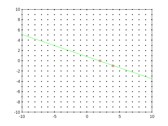
log2(3.6) = p + log2(5)*q
it represents a line in the (p,q) plane, and we want to find a point on the integer lattice (p,q) where the line passes as closely as possible.
[Xl,Yl] = meshgrid([-10:10]);
plot(Xl,Yl,'k.')
hold on
fimplicit(@(p,q) -log2(3.6) + p + log2(5)*q,[-10,10,-10,10],'g-')
plot([2 4],[0,-1],'ro')
hold off
Now, some might think in terms of orthogonal distance to the line, but really, we want the vertical distance to be minimized. Again, minimize abs(delta) in the equation:
log2(3.6) + delta = p + log2(5)*q
where p and q are integer.
Can we do that using MATLAB? The skill about about mathematics often lies in formulating a word problem, and then turning the word problem into a problem of mathematics that we know how to solve. We are almost there now. I next want to formulate this into a problem that intlinprog can solve. The problem at first is intlinprog cannot handle absolute value constraints. And the trick there is to employ slack variables, a terribly useful tool to emply on this class of problem.
Rewrite delta as:
delta = Dpos - Dneg
where Dpos and Dneg are real variables, but both are constrained to be positive.
prob = optimproblem;
p = optimvar('p',lower = -50,upper = 50,type = 'integer');
q = optimvar('q',lower = -50,upper = 50,type = 'integer');
Dpos = optimvar('Dpos',lower = 0);
Dneg = optimvar('Dneg',lower = 0);
Our goal for the ILP solver will be to minimize Dpos + Dneg now. But since they must both be positive, it solves the min absolute value objective. One of them will always be zero.
r = 3.6;
prob.Constraints = log2(r) + Dpos - Dneg == p + log2(5)*q;
prob.Objective = Dpos + Dneg;
The solve is now a simple one. I'll tell it to use intlinprog, even though it would probably figure that out by itself. (Note: if I do not tell solve which solver to use, it does use intlinprog. But it also finds the correct solution when I told it to use GA offline.)
solve(prob,solver = 'intlinprog')
The solution it finds within the bounds of +/- 50 for both p and q seems pretty good. Note that Dpos and Dneg are pretty close to zero.
2^39*5^-16
and while 3.6028979... seems like nothing special, in fact, it is of the form we want.
R = sym(2)^39*sym(5)^-16
vpa(R,100)
vpa(1/R,100)
both of those numbers are exact. If I wanted to find a better approximation to 3.6, all I need do is extend the bounds on p and q. And we can use the same solution approch for any floating point number.
Check out how these charts were made with polar axes in the Graphics and App Building blog's latest article "Polar plots with patches and surface".

Nine new Image Processing courses plus one new learning path are now available as part of the Online Training Suite. These courses replace the content covered in the self-paced course Image Processing with MATLAB, which sunsets in 2026.
New courses include:
- Work with Image Data Types
- Image Registration
- Edge, Circle, and Line Detection
- Manage and Process Multiple Images
The new learning path Image Segmentation and Analysis in MATLAB earns users the digital credential Image Segmentation in MATLAB and contains the following courses:
Timeseries viewer does not open timeseries anymore in 2025a version. Is there any entry level way for the first time users (other that export to Execl file) to show timeseries from all Simulink outport signals as a table? When I teach students who are supposed to use Simulink first time and do not have Matlab experiences, showing data which was created againts time points is quite crucial. But if we have to built separate tables of each outport signal and try to align them to the Editor area it will be embarrasing. But I haven't found any working solution to this simple problem. This was not a problem untill 2025a version came.
Do you have a swag signed by Brian Douglas? He does!
Apparently, the back end here is running 2025b, hovering over the Run button and the Executing In popup both show R2024a.
ver matlab
all(logical.empty)
Discuss!
Issue: PMSM FOC – Flux Weakening Region Current Optimization
I’m using Motor Control Blockset (R2025b) for FOC of a PMSM and facing mismatches in flux-weakening operation compared to MotorCAD/MCIS data.
- Motor setup: 5 pole pairs, Rs = 0.01125 Ω, Ld = 178 µH, Lq = 224 µH, flux = 0.03696 Wb, Vdc = 100 V.
- At low speed (MTPA region): MATLAB’s Id/Iq match MotorCAD well (e.g., 60 Nm @ 1000 rpm).
- At high speed (FW, e.g., 15 Nm @ 7000 rpm): MATLAB selects much higher |Id|, leading to phase currents ≈ 154–161 A, while MotorCAD optimizes at ≈ 96 A. This results in significantly higher copper losses and lower efficiency.
- Tried:
- Single-data model (constant Ld, Lq, flux) → overestimates FW depth.
- LUT-based model (imported MotorCAD Ld/Lq/Flux maps with mcbGenerateTables, idiqLUTs, vclmt method) → closer, but still higher currents vs MotorCAD’s MTPV points.
- Verified constraints (current circle, voltage ellipse, torque hyperbola).
Ask:
How can I configure the PMSM Control Reference block (or supporting functions) to follow MotorCAD’s minimum-current MTPV trajectory in the FW region? Is this a modeling limitation, or do I need custom optimization (e.g., using Model-Based Calibration Toolbox or MotorCAD-MATLAB co-simulation)? Any examples or best practices for accurate FW LUT import would be very helpful.
I just noticed that MATLAB R2025b is available. I am a bit surprised, as I never got notification of the beta test for it.
This topic is for highlights and experiences with R2025b.
For some time now, this has been bugging me - so I thought to gather some more feedback/information/opinions on this.
What would you classify Recursion? As a loop or as a vectorized section of code?
For context, this query occured to me while creating Cody problems involving strict (so to speak) vectorization - (Everyone is more than welcome to check my recent Cody questions).
To make problems interesting and/or difficult, I (and other posters) ban functions and functionalities - such as for loops, while loops, if-else statements, arrayfun() and the rest of the fun() family functions. However, some of the solutions including the reference solution I came up with for my latest problem, contained recursion.
I am rather divided on how to categorize it. What do you think?
I came across this fun video from @Christoper Lum, and I have to admit—his MathWorks swag collection is pretty impressive! He’s got pieces I even don’t have.
So now I’m curious… what MathWorks swag do you have hiding in your office or closet?
- Which one is your favorite?
- Which ones do you want to add to your collection?
Show off your swag and share it with the community! 🚀
Hello!
After updating to MATLAB 2025a, I've noticed a significant decrease in performance when interacting with figures. Specifically, zooming, panning, and other figure manipulations are very slow and occasionally cause the program to freeze.
I often work with complex plots that include multiple tabs and numerous subplots, which means a large amount of data is being displayed. While I acknowledge this is a data-intensive use case, performance in previous MATLAB versions was much smoother.
I'm wondering if anyone else has experienced similar issues since the 2025a update?
It appears that my integrated UHD graphics is being used as the renderer device, despite my laptop having a dedicated NVIDIA GeForce GPU. Are there any settings I can adjust to force MATLAB to use my dedicated GPU for rendering to improve performance?

Any insights or potential solutions would be greatly appreciated! Thank you.
“Hello, I am Subha & I’m part of the organizing/mentoring team for NASA Space Apps Challenge Virudhunagar 2025 🚀. We’re looking for collaborators/mentors with ML and MATLAB expertise to help our student teams bring their space solutions to life. Would you be open to guiding us, even briefly? Your support could impact students tackling real NASA challenges. 🌍✨”
Since R2024b, a Levenberg–Marquardt solver (TrainingOptionsLM) was introduced. The built‑in function trainnet now accepts training options via the trainingOptions function (https://www.mathworks.com/help/deeplearning/ref/trainingoptions.html#bu59f0q-2) and supports the LM algorithm. I have been curious how to use it in deep learning, and the official documentation has not provided a concrete usage example so far. Below I give a simple example to illustrate how to use this LM algorithm to optimize a small number of learnable parameters.
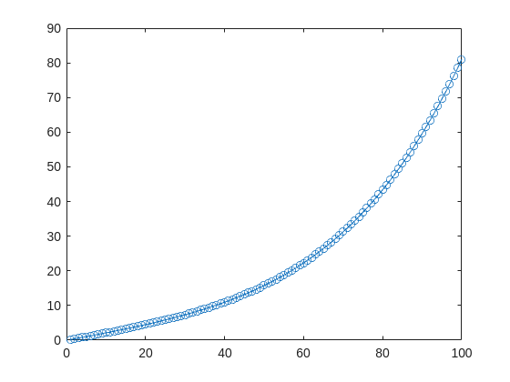
For example, consider the nonlinear function:
y_hat = @(a,t) a(1)*(t/100) + a(2)*(t/100).^2 + a(3)*(t/100).^3 + a(4)*(t/100).^4;
It represents a curve. Given 100 matching points (t → y_hat), we want to use least squares to estimate the four parameters a1–a4.
t = (1:100)';
y_hat = @(a,t)a(1)*(t/100) + a(2)*(t/100).^2 + a(3)*(t/100).^3 + a(4)*(t/100).^4;
x_true = [ 20 ; 10 ; 1 ; 50 ];
y_true = y_hat(x_true,t);
plot(t,y_true,'o-')
- Using the traditional lsqcurvefit-wrapped "Levenberg–Marquardt" algorithm:
x_guess = [ 5 ; 2 ; 0.2 ; -10 ];
options = optimoptions("lsqcurvefit",Algorithm="levenberg-marquardt",MaxFunctionEvaluations=800);
[x,resnorm,residual,exitflag] = lsqcurvefit(y_hat,x_guess,t,y_true,-50*ones(4,1),60*ones(4,1),options);
x,resnorm,exitflag
- Using the deep-learning-wrapped "Levenberg–Marquardt" algorithm:
options = trainingOptions("lm", ...
InitialDampingFactor=0.002, ...
MaxDampingFactor=1e9, ...
DampingIncreaseFactor=12, ...
DampingDecreaseFactor=0.2,...
GradientTolerance=1e-6, ...
StepTolerance=1e-6,...
Plots="training-progress");
numFeatures = 1;
layers = [featureInputLayer(numFeatures,'Name','input')
fitCurveLayer(Name='fitCurve')];
net = dlnetwork(layers);
XData = dlarray(t);
YData = dlarray(y_true);
netTrained = trainnet(XData,YData,net,"mse",options);
netTrained.Layers(2)
classdef fitCurveLayer < nnet.layer.Layer ...
& nnet.layer.Acceleratable
% Example custom SReLU layer.
properties (Learnable)
% Layer learnable parameters
a1
a2
a3
a4
end
methods
function layer = fitCurveLayer(args)
arguments
args.Name = "lm_fit";
end
% Set layer name.
layer.Name = args.Name;
% Set layer description.
layer.Description = "fit curve layer";
end
function layer = initialize(layer,~)
% layer = initialize(layer,layout) initializes the layer
% learnable parameters using the specified input layout.
if isempty(layer.a1)
layer.a1 = rand();
end
if isempty(layer.a2)
layer.a2 = rand();
end
if isempty(layer.a3)
layer.a3 = rand();
end
if isempty(layer.a4)
layer.a4 = rand();
end
end
function Y = predict(layer, X)
% Y = predict(layer, X) forwards the input data X through the
% layer and outputs the result Y.
% Y = layer.a1.*exp(-X./layer.a2) + layer.a3.*X.*exp(-X./layer.a4);
Y = layer.a1*(X/100) + layer.a2*(X/100).^2 + layer.a3*(X/100).^3 + layer.a4*(X/100).^4;
end
end
end
The network is very simple — only the fitCurveLayer defines the learnable parameters a1–a4. I observed that the output values are very close to those from lsqcurvefit.
I saw this YouTube short on my feed: What is MATLab?

I was mostly mesmerized by the minecraft gameplay going on in the background.
Found it funny, thought i'd share.
Can MATLAB be used to design a liquid ejector? For example, given the pressure and flow rate of water at the ejector inlet and the suction port, how can the relevant structural dimensions of the ejector be calculated?