Results for
Experimenting with Agentic AI
44%
I am an AI skeptic
0%
AI is banned at work
11%
I am happy with Conversational AI
44%
9 votes
The Cody Contest 2025 is underway, and it includes a super creative problem group which many of us have found fascinating. The central theme of the problems, expertly curated by @Matt Tearle, humorously revolves around the whims of the capricious dictator Lord Ned, as he goes out of his way to complicate the lives of his subjects and visitors alike. We cannot judge whether or not there's any truth to the rumors behind all the inside jokes, but it's obvious that the team had a lot of fun creating these; and we had even more fun solving them.
Today I want to showcase a way of graphically solving and visualizing one of those problems which I found very elegant, The Bridges of Nedsburg.
To briefly reiterate the problem, the number of islands and the arrangement of bridges of the city of Nedsburg are constantly changing. Lord Ned has decided to take advantage of this by charging visitors with an increasingly expensive n-bridge pass which allows them to cross up to n bridges in one journey. Given the Connectivity Matrix C, we are tasked with calculating the minimum n needed so that there is a path from every island to every other island in n steps or fewer.
Matt kindly provided us with some useful bit of math in the description detailing how to calculate the way to get from one island to another in an number of m steps. However, he has also hidden an alternative path to the solution in plain sight, in one of the graphs he provided. This involves the extremely useful and versatile class digraph, representing directed graphs, which have directional edges connecting the nodes. Here's some further great documentation and other cool resources on the topic for those who are interested in learning more about it:
Let's start using this class to explore a graphical solution to Lord Ned's conundrum. We will use the unit tests included in the problem to visualize the solution. We can retrieve the connectivity matrix for each case using the following function:
function C = getConnectivityMatrix(unit_test)
% Number of islands and bridge arrangement
switch unit_test
case 1
m = 3; idx = [3;4;8];
case 2
m = 3; idx = [3;4;7;8];
case 3
m = 4; idx = [2;7;8;10;13];
case 4
m = 4; idx = [4;5;7;8;9;14];
case 5
m = 5; idx = [5;8;11;12;14;18;22;23];
case 6
m = 5; idx = [2;5;8;14;20;21;24];
case 7
m = 6; idx = [3;4;7;11;18;23;24;26;30;32];
case 8
m = 6; idx = [3;11;12;13;18;19;28;32];
case 9
m = 7; idx = [3;4;6;8;13;14;20;21;23;31;36;47];
case 10
m = 7; idx = [4;11;13;14;19;22;23;26;28;30;34;35;37;38;45];
case 11
m = 8; idx = [2;4;5;6;8;12;13;17;27;39;44;48;54;58;60;62];
case 12
m = 8; idx = [3;9;12;20;24;29;30;31;33;44;48;50;53;54;58];
case 13
m = 9; idx = [8;9;10;14;15;22;25;26;29;33;36;42;44;47;48;50;53;54;55;67;80];
case 14
m = 9; idx = [8;10;22;32;37;40;43;45;47;53;56;57;62;64;69;70;73;77;79];
case 15
m = 10; idx = [2;5;8;13;16;20;24;27;28;36;43;49;53;62;71;75;77;83;86;87;95];
case 16
m = 10; idx = [4;9;14;21;22;35;37;38;44;47;50;51;53;55;59;61;63;66;69;76;77;84;85;86;90;97];
end
C = zeros(m);
C(idx) = 1;
end
The case in the example refers to unit test case 2.
unit_test = 2;
C = getConnectivityMatrix(unit_test);
disp(C)
D = digraph(C);
figure
p = plot(D,'LineWidth',1.5,'ArrowSize',10);
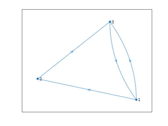
This is the same as the graph provided in the example. Another very useful method of digraph is shortestpath. This allows us to calculate the path and distance from one single node to another. For example:
% Path and distance from node 1 to node 2
[path12,dist12] = shortestpath(D,1,2);
fprintf('The shortest path from island %d to island %d is: %s. The minimum number of steps is: n = %d\n', 1, 2, join(string(path12), ' -> '),dist12)
% Path and distance from node 2 to node 1
[path21,dist21] = shortestpath(D,2,1);
fprintf('The shortest path from island %d to island %d is: %s. The minimum number of steps is: n = %d\n', 2, 1, join(string(path21), ' -> '),dist21)
figure
p = plot(D,'LineWidth',1.5,'ArrowSize',10);
highlight(p,path12,'EdgeColor','r','NodeColor','r','LineWidth',2)
highlight(p,path21,'EdgeColor',[0 0.8 0],'LineWidth',2)

But that's not all! digraph can also provide us with a matrix of the distances d, i.e. the steps needed to travel from island i to island j, where i and j are the rows and columns of d respectively. This is accomplished by using its distances method. The distance matrix can be visualized as:
d = distances(D);
figure
% Using pcolor w/ appending matrix workaround for convenience
pcolor([d,d(:,end);d(end,:),d(end,end)])
% Alternatively you can use imagesc(d), but you'll have to recreate the grid manually
axis square
set(gca,'YDir','reverse','XTick',[],'YTick',[])
[X,Y] = meshgrid(1:height(d));
text(X(:)+0.5,Y(:)+0.5,string(d(:)),'FontSize',11)
colormap(interp1(linspace(0,1,4), [1 1 1; 0.7 0.9 1; 0.6 0.7 1; 1 0.3 0.3], linspace(0,1,8)))
clim([-0.5 7+0.5])
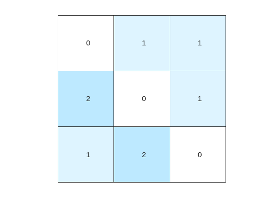
This confirms what we saw before, i.e. you need 1 step to go from island 1 to island 2, but 2 steps for vice versa. It also confirms that the minimum number of steps n that you need to buy the pass for is 2 (which also occurs for traveling from island 3 to island 2). As it's not the point of the post to give the full solution to the problem but rather present the graphical way of visualizing it I will not include the code of how to calculate this, but I'm sure that by now it's reduced to a trivial problem which you have already figured out how to solve.
That being said, now that we have the distance matrix, let's continue with the visualizations. First, let's plot the corresponding paths for each of these combinations:
figure
tiledlayout(size(C,1),size(C,2),'TileSpacing','tight','Padding','tight');
for i = 1:size(C,1)
for j = 1:size(C,2)
nexttile
p = plot(D,'ArrowSize',10);
highlight(p,shortestpath(D,i,j),'EdgeColor','r','NodeColor','r','LineWidth',2)
lims = axis;
text(lims(1)+diff(lims(1:2))*0.05,lims(3)+diff(lims(3:4))*0.9,sprintf('n = %d',d(i,j)))
end
end

This allows us to go from the distance matrix to visualizing the paths and number of steps for each corresponding case. Things are rather simple for this 3-island example case, but evil Lord Ned is just getting started. Let's now try to solve the problem for all provided unit test cases:
% Cell array of connectivity matrices
C = arrayfun(@getConnectivityMatrix,1:16,'UniformOutput',false);
% Cell array of corresponding digraph objects
D = cellfun(@digraph,C,'UniformOutput',false);
% Cell array of corresponding distance matrices
d = cellfun(@distances,D,'UniformOutput',false);
% id of solutions: Provided as is to avoid handing out the code to the full solution
id = [2, 2, 9, 3, 4, 6, 16, 4, 44, 43, 33, 34, 7, 18, 39, 2];
First, let's plot the distance matrix for each case:
figure
tiledlayout('flow','TileSpacing','compact','Padding','compact');
% Vary this to plot different combinations of cases
plot_cases = 1:numel(C);
for i = plot_cases
nexttile
pcolor([d{i},d{i}(:,end);d{i}(end,:),d{i}(end,end)])
axis square
set(gca,'YDir','reverse','XTick',[],'YTick',[])
title(sprintf('Case %d',i),'FontWeight','normal','FontSize',8)
end
c = colorbar('Ticks',0:7,'TickLength',0,'Limits',[-0.5 7+0.5],'FontSize',8);
c.Layout.Tile = 'East';
c.Label.String = 'Number of Steps';
c.Label.FontSize = 8;
colormap(interp1(linspace(0,1,4), [1 1 1; 0.7 0.9 1; 0.6 0.7 1; 1 0.3 0.3], linspace(0,1,8)))
clim(findobj(gcf,'type','axes'),[-0.5 7+0.5])
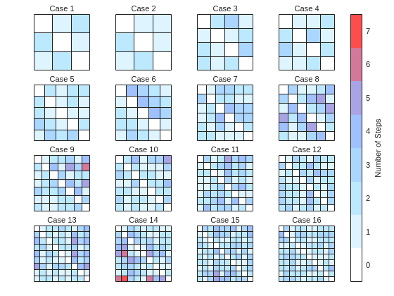
We immediately notice some inconsistencies, perhaps to be expected of the eccentric and cunning dictator. Things are pretty simple for the configurations with a small number of islands, but the minimum number of steps n can increase sharply and disproportionally to the additional number of islands. Cases 8 and 9 specifically have a particularly large n (relative to their grid dimensions), and case 14 has the largest n, almost double that of case 16 despite the fact that the latter has one extra island.
To visualize how this is possible, let's plot the path corresponding to the largest n for each case (though note that there might be multiple possible paths for each case):
figure
tiledlayout('flow','TileSpacing','tight','Padding','tight');
for i = plot_cases
nexttile
% Changing the layout to circular so we can better visualize the paths
p = plot(D{i},'ArrowSize',10,'Layout','Circle');
% Alternatively we could use the XData and YData properties if the positions of the islands were provided
axis([-1.5 1.5 -1.5 1.75])
[row,col] = ind2sub(size(d{i}),id(i));
highlight(p,shortestpath(D{i},row,col),'EdgeColor','r','NodeColor','r','LineWidth',2)
lims = axis;
text(lims(1)+diff(lims(1:2))*0.05,lims(3)+diff(lims(3:4))*0.9,sprintf('n = %d',d{i}(row,col)))
end
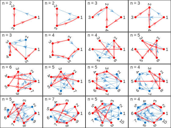
And busted! Unraveled! Exposed! Lord Ned has clearly been taking advantages of the tectonic forces by instructing his corrupt civil engineer lackeys to design the bridges to purposely force the visitors to go around in circles in order to drain them of their precious savings. In particular, for cases 8 and 9, he would have them go through every single island just to get from one island to another, whereas for case 14 they would have to visit 8 of the 9 islands just to get to their destination. If that's not diabolical then I don't know what is!
Ned jokes aside, I hope you enjoyed this contest just as much as I did, and that you found this article useful. I look forward to seeing more creative problems and solutions in the future.

It’s exciting to dive into a new dataset full of unfamiliar variables but it can also be overwhelming if you’re not sure where to start. Recently, I discovered some new interactive features in MATLAB live scripts that make it much easier to get an overview of your data. With just a few clicks, you can display sparklines and summary statistics using table variables, sort and filter variables, and even have MATLAB generate the corresponding code for reproducibility.
The Graphics and App Building blog published an article that walks through these features showing how to explore, clean, and analyze data—all without writing any code.
If you’re interested in streamlining your exploratory data analysis or want to see what’s new in live scripts, you might find it helpful:
If you’ve tried these features or have your own tips for quick data exploration in MATLAB, I’d love to hear your thoughts!
I am Prof Ansar Interested in coding challenge taker inmatlab
What a fantastic start to Cody Contest 2025! In just 2 days, over 300 players joined the fun, and we already have our first contest group finishers. A big shoutout to the first finisher from each team:
- Team Creative Coders: @Mehdi Dehghan
- Team Cool Coders: @Pawel
- Team Relentless Coders: @David Hill
- 🏆 First finisher overall: Mehdi Dehghan
Other group finishers: @Bin Jiang (Relentless), @Mazhar (Creative), @Vasilis Bellos (Creative), @Stefan Abendroth (Creative), @Armando Longobardi (Cool), @Cephas (Cool)
Kudos to all group finishers! 🎉
Reminder to finishers: The goal of Cody Contest is learning together. Share hints (not full solutions) to help your teammates complete the problem group. The winning team will be the one with the most group finishers — teamwork matters!
To all players: Don’t be shy about asking for help! When you do, show your work — include your code, error messages, and any details needed for others to reproduce your results.
Keep solving, keep sharing, and most importantly — have fun!
Title: Looking for Internship Guidance as a Beginner MATLAB/Simulink Learner
Hello everyone,
I’m a Computer Science undergraduate currently building a strong foundation in MATLAB and Simulink. I’m still at a beginner level, but I’m actively learning every day and can work confidently once I understand the concepts. Right now I’m focusing on MATLAB modeling, physics simulation, and basic control systems so that I can contribute effectively to my current project.
I’m part of an Autonomous Underwater Vehicle (AUV) team preparing for the Singapore AUV Challenge (SAUVC). My role is in physics simulation, controls, and navigation, and MATLAB/Simulink plays a major role in that pipeline. I enjoy physics and mathematics deeply, which makes learning modeling and simulation very exciting for me.
On the coding side, I practice competitive programming regularly—
• Codeforces rating: ~1200
• LeetCode rating: ~1500
So I'm comfortable with logic-building and problem solving. What I’m looking for:
I want to know how a beginner like me can start applying for internships related to MATLAB, Simulink, modeling, simulation, or any engineering team where MATLAB is widely used (including companies outside MathWorks).
I would really appreciate advice from the community on:
- What skills should I strengthen first?
- Which MATLAB/Simulink toolboxes are most important for beginners aiming toward simulation/control roles?
- What small projects or portfolio examples should I build to improve my profile?
- What is the best roadmap to eventually become a good candidate for internships in this area?
Any guidance, resources, or suggestions would be extremely helpful for me.
Thank you in advance to everyone who shares their experience!
The main round of Cody Contest 2025 kicks off today! Whether you’re a beginner or a seasoned solver, now’s your time to shine.
Here’s how to join the fun:
- Pick your team — choose one that matches your coding personality.
- Solve Cody problems — gain points and climb the leaderboard.
- Finish the Contest Problem Group — help your team win and unlock chances for weekly prizes by finishing the Cody Contest 2025 problem group.
- Share Tips & Tricks — post your insights to win a coveted MathWorks Yeti Bottle.
- Bonus Round — 2 players from each team will be invited to a fun live code-along event!
- Watch Party – join the big watch event to see how top players tackle Cody problems
Contest Timeline:
- Main Round: Nov 10 – Dec 7, 2025
- Bonus Round: Dec 8 – Dec 19, 2025
Big prizes await — MathWorks swag, Amazon gift cards, and shiny virtual badges!
We look forward to seeing you in the contest — learn, compete, and have fun!
Parallel Computing Onramp is here! This free, one-hour self-paced course teaches the basics of running MATLAB code in parallel using multiple CPU cores, helping users speed up their code and write code that handles information efficiently.
Remember, Onramps are free for everyone - give the new course a try if you're curious. Let us know what you think of it by replying below.
Run MATLAB using AI applications by leveraging MCP. This MCP server for MATLAB supports a wide range of coding agents like Claude Code and Visual Studio Code.
Check it out and share your experiences below. Have fun!
GitHub repo: https://github.com/matlab/matlab-mcp-core-server
Yann Debray's blog post: https://blogs.mathworks.com/deep-learning/2025/11/03/releasing-the-matlab-mcp-core-server-on-github/
Hey Creative Coders! 😎
Let’s get to know each other. Drop a quick intro below and meet your teammates! This is your chance to meet teammates, find coding buddies, and build connections that make the contest more fun and rewarding!
You can share:
- Your name or nickname
- Where you’re from
- Your favorite coding topic or language
- What you’re most excited about in the contest
Let’s make Team Creative Coders an awesome community—jump in and say hi! 🚀
Welcome to the Cody Contest 2025 and the Creative Coders team channel! 🎉
You think outside the box. Where others see limitations, you see opportunities for innovation. This is your space to connect with like-minded coders, share insights, and help your team win. To make sure everyone has a great experience, please keep these tips in mind:
- Follow the Community Guidelines: Take a moment to review our community standards. Posts that don’t follow these guidelines may be flagged by moderators or community members.
- Ask Questions About Cody Problems: When asking for help, show your work! Include your code, error messages, and any details needed to reproduce your results. This helps others provide useful, targeted answers.
- Share Tips & Tricks: Knowledge sharing is key to success. When posting tips or solutions, explain how and why your approach works so others can learn your problem-solving methods.
- Provide Feedback: We value your feedback! Use this channel to report issues or share creative ideas to make the contest even better.
Have fun and enjoy the challenge! We hope you’ll learn new MATLAB skills, make great connections, and win amazing prizes! 🚀
как я получил api Token
I am excited to join this community to learn the more particularly the Matlab/Simulink
I just learned you can access MATLAB Online from the following shortcut in your web browser: https://matlab.new
Thanks @Yann Debray
From his recent blog post: pip & uv in MATLAB Online » Artificial Intelligence - MATLAB & Simulink
I'm developing a comprehensive MATLAB programming course and seeking passionate co-trainers to collaborate!
Why MATLAB Matters:Many people underestimate MATLAB's significance in:
- Communication systems
- Signal processing
- Mathematical modeling
- Engineering applications
- Scientific computing
Course Structure:
- Foundation Module: MATLAB basics and fundamentals
- Image Processing: Practical applications and techniques
- Signal Processing: Analysis and implementation
- Machine Learning: ML algorithms using MATLAB
- Hands-on Learning: Projects, assignments.
What I'm Looking For:
- Enthusiastic educators willing to share knowledge
- Experience in any MATLAB application area
- Commitment to collaborative teaching
Interested in joining as a co-trainer? Please comment below or reach out directly!
Online Doc + System Browser
11%
Online Doc + Dedicated Browser
11%
Offline Doc +System Browser
11%
Offline Doc + Dedicated Browser
23%
Hybrid Approach (Support All Modes)
23%
User-Definable / Fully Configurable
20%
35 votes
Hey everyone,
I’m currently working with MATLAB R2025b and using the MQTT blocks from the Industrial Communication Toolbox inside Simulink. I’ve run into an issue that’s driving me a bit crazy, and I’m not sure if it’s a bug or if I’m missing something obvious.
Here’s what’s happening:
- I open the MQTT Configure block.
- I fill out all the required fields — Broker address, Port, Client ID, Username, and Password.
- When I click Test Connection, it says “Connection established successfully.” So far so good.
- Then I click Apply, close the dialog, set the topic name, and try to run the simulation.
- At this point, I get the following error:Caused by: Invalid value for 'ClientID', 'Username' or 'Password'.
- When I reopen the MQTT config block, I notice that the Password field is empty again — even though I definitely entered it before and the connection test worked earlier.
It seems like Simulink is somehow not saving the password after hitting Apply, which leads to the authentication error during simulation.
Has anyone else faced this? Is this a bug in R2025b, or do I need to configure something differently to make the password persist?
Would really appreciate any insights, workarounds, or confirmations from anyone who has used MQTT in Simulink recently.
Thanks in advance!
I recently published this blog post about resources to help people learn MATLAB https://blogs.mathworks.com/matlab/2025/09/11/learning-matlab-in-2025/
What are your favourite MATLAB learning resources?
What if you had no isprime utility to rely on in MATLAB? How would you identify a number as prime? An easy answer might be something tricky, like that in simpleIsPrime0.
simpleIsPrime0 = @(N) ismember(N,primes(N));
But I’ll also disallow the use of primes here, as it does not really test to see if a number is prime. As well, it would seem horribly inefficient, generating a possibly huge list of primes, merely to learn something about the last member of the list.
Looking for a more serious test for primality, I’ve already shown how to lighten the load by a bit using roughness, to sometimes identify numbers as composite and therefore not prime.
https://www.mathworks.com/matlabcentral/discussions/tips/879745-primes-and-rough-numbers-basic-ideas
But to actually learn if some number is prime, we must do a little more. Yes, this is a common homework problem assigned to students, something we have seen many times on Answers. It can be approached in many ways too, so it is worth looking at the problem in some depth.
The definition of a prime number is a natural number greater than 1, which has only two factors, thus 1 and itself. That makes a simple test for primality of the number N easy. We just try dividing the number by every integer greater than 1, and not exceeding N-1. If any of those trial divides leaves a zero remainder, then N cannot be prime. And of course we can use mod or rem instead of an explicit divide, so we need not worry about floating point trash, as long as the numbers being tested are not too large.
simpleIsPrime1 = @(N) all(mod(N,2:N-1) ~= 0);
Of course, simpleIsPrime1 is not a good code, in the sense that it fails to check if N is an integer, or if N is less than or equal to 1. It is not vectorized, and it has no documentation at all. But it does the job well enough for one simple line of code. There is some virtue in simplicity after all, and it is certainly easy to read. But sometimes, I wish a function handle could include some help comments too! A feature request might be in the offing.
simpleIsPrime1(9931)
simpleIsPrime1(9932)
simpleIsPrime1 works quite nicely, and seems pretty fast. What could be wrong? At some point, the student is given a more difficult problem, to identify if a significantly larger integer is prime. simpleIsPrime1 will then cause a computer to grind to a distressing halt if given a sufficiently large number to test. Or it might even error out, when too large a vector of numbers was generated to test against. For example, I don't think you want to test a number of the order of 2^64 using simpleIsPrime1, as performing on the order of 2^64 divides will be highly time consuming.
uint64(2)^63-25
Is it prime? I’ve not tested it to learn if it is, and simpleIsPrime1 is not the tool to perform that test anyway.
A student might realize the largest possible integer factors of some number N are the numbers N/2 and N itself. But, if N/2 is a factor, then so is 2, and some thought would suggest it is sufficient to test only for factors that do not exceed sqrt(N). This is because if a is a divisor of N, then so is b=N/a. If one of them is larger than sqrt(N), then the other must be smaller. That could lead us to an improved scheme in simpleIsPrime2.
simpleIsPrime2 = @(N) all(mod(N,2:sqrt(N)));
For an integer of the size 2^64, now you only need to perform roughly 2^32 trial divides. Maybe we might consider the subtle improvement found in simpleIsPrime3, which avoids trial divides by the even integers greater than 2.
simpleIsPrime3 = @(N) (N == 2) || (mod(N,2) && all(mod(N,3:2:sqrt(N))));
simpleIsPrime3 needs only an approximate maximum of 2^31 trial divides even for numbers as large as uint64 can represent. While that is large, it is still generally doable on the computers we have today, even if it might be slow.
Sadly, my goals are higher than even the rather lofty limit given by UINT64 numbers. The problem of course is that a trial divide scheme, despite being 100% accurate in its assessment of primality, is a time hog. Even an O(sqrt(N)) scheme is far too slow for numbers with thousands or millions of digits. And even for a number as “small” as 1e100, a direct set of trial divides by all primes less than sqrt(1e100) would still be practically impossible, as there are roughly n/log(n) primes that do not exceed n. For an integer on the order of 1e50,
1e50/log(1e50)
It is practically impossible to perform that many divides on any computer we can make today. Can we do better? Is there some more efficient test for primality? For example, we could write a simple sieve of Eratosthenes to check each prime found not exceeding sqrt(N).
function [TF,SmallPrime] = simpleIsPrime4(N)
% simpleIsPrime3 - Sieve of Eratosthenes to identify if N is prime
% [TF,SmallPrime] = simpleIsPrime3(N)
%
% Returns true if N is prime, as well as the smallest prime factor
% of N when N is composite. If N is prime, then SmallPrime will be N.
Nroot = ceil(sqrt(N)); % ceil caters for floating point issues with the sqrt
TF = true;
SieveList = true(1,Nroot+1); SieveList(1) = false;
SmallPrime = 2;
while TF
% Find the "next" true element in SieveList
while (SmallPrime <= Nroot+1) && ~SieveList(SmallPrime)
SmallPrime = SmallPrime + 1;
end
% When we drop out of this loop, we have found the next
% small prime to check to see if it divides N, OR, we
% have gone past sqrt(N)
if SmallPrime > Nroot
% this is the case where we have now looked at all
% primes not exceeding sqrt(N), and have found none
% that divide N. This is where we will drop out to
% identify N as prime. TF is already true, so we need
% not set TF.
SmallPrime = N;
return
else
if mod(N,SmallPrime) == 0
% smallPrime does divide N, so we are done
TF = false;
return
end
% update SieveList
SieveList(SmallPrime:SmallPrime:Nroot) = false;
end
end
end
simpleIsPrime4 does indeed work reasonably well, though it is sometimes a little slower than is simpleIsPrime3, and everything is hugely faster than simpleIsPrime1.
timeit(@() simpleIsPrime1(111111111))
timeit(@() simpleIsPrime2(111111111))
timeit(@() simpleIsPrime3(111111111))
timeit(@() simpleIsPrime4(111111111))
All of those times will slow to a crawl for much larger numbers of course. And while I might find a way to subtly improve upon these codes, any improvement will be marginal in the end if I try to use any such direct approach to primality. We must look in a different direction completely to find serious gains.
At this point, I want to distinguish between two distinct classes of tests for primality of some large number. One class of test is what I might call an absolute or infallible test, one that is perfectly reliable. These are tests where if X is identified as prime/composite then we can trust the result absolutely. The tests I showed in the form of simpleIsPrime1, simpleIsPrime2, simpleIsPrime3 and aimpleIsprime4, were all 100% accurate, thus they fall into the class of infallible tests.
The second general class of test for primality is what I will call an evidentiary test. Such a test provides evidence, possibly quite strong evidence, that the given number is prime, but in some cases, it might be mistaken. I've already offered a basic example of a weak evidentiary test for primality in the form of roughness. All primes are maximally rough. And therefore, if you can identify X as being rough to some extent, this provides evidence that X is also prime, and the depth of the roughness test influences the strength of the evidence for primality. While this is generally a fairly weak test, it is a test nevertheless, and a good exclusionary test, a good way to avoid more sophisticated but time consuming tests.
These evidentiary tests all have the property that if they do identify X as being composite, then they are always correct. In the context of roughness, if X is not sufficiently rough, then X is also not prime. On the other side of the coin, if you can show X is at least (sqrt(X)+1)-rough, then it is positively prime. (I say this to suggest that some evidentiary tests for primality can be turned into truth telling tests, but that may take more effort than you can afford.) The problem is of course that is literally impossible to verify that degree of roughness for numbers with many thousands of digits.
In my next post, I'll look at the Fermat test for primality, based on Fermat's little theorem.