scal2frq
Scale to frequency
Description
Examples
This example shows how the pseudo-frequency changes as you double the scale.
Construct a vector of scales with 10 voices per octave over five octaves.
vpo = 10;
no = 5;
a0 = 2^(1/vpo);
ind = 0:vpo*no;
sc = a0.^ind;
Verify that the range of scales covers five octaves.
log2(max(sc)/min(sc))
ans =
5.0000
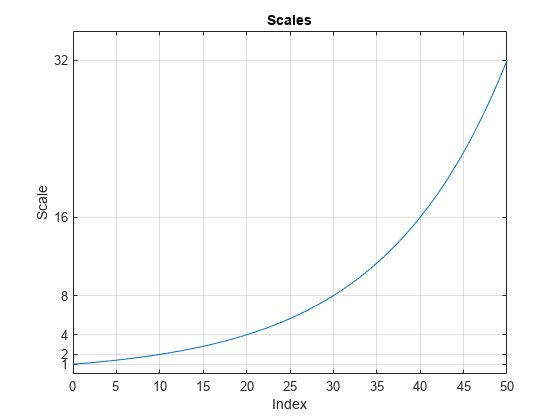
If you plot the scales, you can use a data cursor to confirm that the scale at index is twice the scale at index . Set the y-ticks to mark each octave.
plot(ind,sc)
title('Scales')
xlabel('Index')
ylabel('Scale')
grid on
set(gca,'YTick',2.^(0:5))

Convert the scales to pseudo-frequencies for the real-valued Morlet wavelet. First, assume the sampling period is 1. Since there are 10 voices per octave, display every tenth row in the table. Observe that for each doubling of the scale, the pseudo-frequency is cut in half.
pf = scal2frq(sc,"morl");
T = [sc(:) pf(:)];
T = array2table(T, ...
    'VariableNames',{'Scale','Pseudo-Frequency'});
disp(T(1:10:end,:))
    Scale    Pseudo-Frequency
    _____    ________________

      1            0.8125
      2           0.40625
      4           0.20313
      8           0.10156
     16          0.050781
     32          0.025391
Assume that data is sampled at 100 Hz. Construct a table with the scales, the corresponding pseudo-frequencies, and periods. Display every tenth row in the table.
Fs = 100;
DT = 1/Fs;
pf = scal2frq(sc,"morl",DT);
T = [sc(:)/Fs pf(:) 1./pf(:)];
T = array2table(T, ...
    'VariableNames',{'Scale','Pseudo-Frequency','Period'});
T(1:vpo:end,:)
ans=6×3 table
    Scale    Pseudo-Frequency     Period
    _____    ________________    ________

    0.01           81.25         0.012308
    0.02          40.625         0.024615
    0.04          20.313         0.049231
    0.08          10.156         0.098462
    0.16          5.0781          0.19692
    0.32          2.5391          0.39385
Note the presence of the factor in scal2frq. This is necessary in order to achieve the proper scale-to-frequency conversion. The is needed to adjust the raw scales properly. For example, with:
f = scal2frq(1,'morl',0.01);You are really asking what happens to the center frequency of the mother Morlet wavelet, if you dilate the wavelet by 0.01. In other words, what is the effect on the center frequency if instead of , you look at . The provides the correct adjustment factor on the scales.
You could have obtained the same results by first converting the scales to their adjusted sizes and then using scal2frq without specifying .
scadjusted = sc.*0.01;
pf2 = scal2frq(scadjusted,'morl');
max(pf-pf2)
ans = 0
The example shows how to create a contour plot of the CWT using approximate frequencies in Hz.
Create a signal consisting of two sine waves with disjoint support in additive noise. Assume the signal is sampled at 1 kHz.
Fs = 1000;
t = 0:1/Fs:1-1/Fs;
x = 1.5*cos(2*pi*100*t).*(t<0.25)+1.5*cos(2*pi*50*t).*(t>0.5 & t<=0.75);
x = x+0.05*randn(size(t));
Obtain the CWT of the input signal and plot the result.
[cfs,f] = cwt(x,Fs);
contour(t,f,abs(cfs).^2);
axis tight;
grid on;
xlabel('Time');
ylabel('Approximate Frequency (Hz)');
title('CWT with Time vs Frequency');

Input Arguments
Scales, specified as a positive real-valued vector.
Wavelet, specified as a character vector or string scalar. See wavefun for more
information.
Sampling period, specified as a real-valued scalar.
Example: pf = scal2frq([1:5],"db4",0.01)
More About
There is only an approximate answer for the relationship between scale and frequency.
In wavelet analysis, the way to relate scale to frequency is to determine the center frequency of the wavelet, Fc, and use the following relationship:
where
a is a scale.
Fc is the center frequency of the wavelet in Hz.
Fa is the pseudo-frequency corresponding to the scale a, in Hz.
The idea is to associate with a given wavelet a purely periodic signal of
frequency Fc. The frequency maximizing the
Fourier transform of the wavelet modulus is
Fc. The centfrq function computes the
center frequency for a specified wavelet. From the above relationship, it can be
seen that scale is inversely proportional to pseudo-frequency. For example, if the
scale increases, the wavelet becomes more spread out, resulting in a lower
pseudo-frequency.
Some examples of the correspondence between the center frequency and the wavelet are shown in the following figure.
Center Frequencies for Real and Complex Wavelets

References
[1] Abry, P. Ondelettes et turbulence. Multirésolutions, algorithmes de décomposition, invariance d'échelles et signaux de pression. Diderot, Editeurs des sciences et des arts, Paris, 1997.
Version History
Introduced before R2006a
See Also
MATLAB Command
You clicked a link that corresponds to this MATLAB command:
Run the command by entering it in the MATLAB Command Window. Web browsers do not support MATLAB commands.
Select a Web Site
Choose a web site to get translated content where available and see local events and offers. Based on your location, we recommend that you select: .
You can also select a web site from the following list
How to Get Best Site Performance
Select the China site (in Chinese or English) for best site performance. Other MathWorks country sites are not optimized for visits from your location.
Americas
- América Latina (Español)
- Canada (English)
- United States (English)
Europe
- Belgium (English)
- Denmark (English)
- Deutschland (Deutsch)
- España (Español)
- Finland (English)
- France (Français)
- Ireland (English)
- Italia (Italiano)
- Luxembourg (English)
- Netherlands (English)
- Norway (English)
- Österreich (Deutsch)
- Portugal (English)
- Sweden (English)
- Switzerland
- United Kingdom (English)