Wavelet Synchrosqueezing
What is Wavelet Synchrosqueezing?
The wavelet synchrosqueezed transform is a time-frequency analysis method that is useful for analyzing multicomponent signals with oscillating modes. Examples of signals with oscillating modes include speech waveforms, machine vibrations, and physiologic signals. Many of these real-world signals with oscillating modes can be written as a sum of amplitude-modulated and frequency-modulated components. A general expression for these types of signals with summed components is
where is the slowly varying amplitude and is the instantaneous phase. A truncated Fourier series, where the amplitude and frequency do not vary with time, is a special case of these signals.
The wavelet transform and other linear time-frequency analysis methods decompose these signals into their components by correlating the signal with a dictionary of time-frequency atoms [1]. The wavelet transform uses translated and scaled versions of a mother wavelet as its time-frequency atoms. Some time-frequency spreading is associated with all of these time-frequency atoms, which affects the sharpness of the signal analysis.
The wavelet synchrosqueezed transform is a time-frequency method that reassigns the signal energy in frequency. This reassignment compensates for the spreading effects caused by the mother wavelet. Unlike other time-frequency reassignment methods, synchrosqueezing reassigns the energy only in the frequency direction, which preserves the time resolution of the signal. By preserving the time, the inverse synchrosqueezing algorithm can reconstruct an accurate representation of the original signal. To use synchrosqueezing, each term in the summed components signal expression must be an intrinsic mode type (IMT) function. For details on the criteria that constitute IMTs, see [2].
Wavelet Synchrosqueezing Algorithm
The synchrosqueezing algorithm uses these steps.
Choose an analytic wavelet . For use with synchrosqueezing, the CWT must use a complex-valued wavelet to capture instantaneous frequency information.
Use the wavelet to obtain the CWT of the input signal : . The variables s and u denote the scale and translation parameters respectively.
Extract the instantaneous frequencies from the CWT output, using a phase transform, . This phase transform is proportional to the first derivative of the CWT with respect to u.
The scales are defined as , where is the peak frequency of the wavelet and ω is the frequency.
“Squeeze” the CWT over regions where the phase transform is constant. The resulting instantaneous frequency value is reassigned to a single value at the centroid of the CWT time-frequency region. This reassignment results in sharpened output from the synchrosqueezed transform when compared to the CWT.
As described, synchrosqueezing uses the continuous wavelet transform (CWT) and its first derivative with respect to translation. The CWT is invertible and since the synchrosqueezed transform inherits the CWT invertibility property, the signal can be reconstructed.
Illustration: Instantaneous Frequency Extraction
You can express the CWT of the function with respect to the wavelet in terms of the inverse Fourier transform of the product of the function's Fourier transform and the wavelet's Fourier transform:
where the bar over denotes complex conjugate.
Consider a simple complex exponential, . To extract the instantaneous frequency of :
Obtain the wavelet transform of the function:
where is the Fourier transform of the wavelet at .
Take the partial derivative of the previous equation with respect to the translation, u:
Apply the definition of the phase transform (step 3 in Wavelet Synchrosqueezing Algorithm) to obtain the instantaneous frequency: .
Required Component Separation
With synchrosqueezing the signal components must be IMTs that are well separated in the
time-frequency plane. If this requirement is met, you can track the trajectory of the
instantaneous frequencies along a curve. The curves show the location of the maximum energy
as it varies over time for each signal mode. See wsstridge for a description of the trajectory curves algorithm.
This inequality defines the required separation criteria:
where is the instantaneous frequency and d is a positive separation constant [2]. To determine this required separation, suppose a bump wavelet, x, has a Fourier transform with support in the range . Because the bump wavelet has a center frequency of Hz, use as the interval. Then solve for d to get for the bump wavelet.
To show this separation requirement for the bump wavelet, consider a signal composed of . Using the bump wavelet to obtain the CWT, the instantaneous phase of the cosine is , and the instantaneous frequency is the first derivative, 0.1. Likewise, for the sine component, the instantaneous frequency is 0.2. The separation inequality, , is true. Therefore, the two signal components are IMT functions and are separated enough to use the synchrosqueezed transform.
If you use higher frequencies, such as 0.3 and 0.4 for the instantaneous frequencies, the inequality is , which is not true. Because these signal components are not well-separated IMTs the signal, , is not appropriate for use with the synchrosqueezed transform.
Examples
CWT vs Synchrosqueezed Transform Smearing
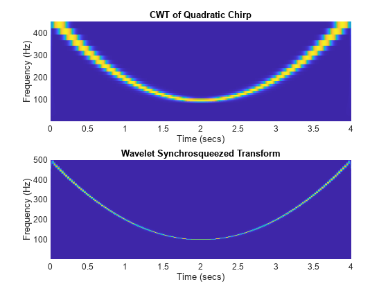
Comparing the CWT with the synchrosqueezed transform of a quadratic chirp shows reduced energy smearing for the synchrosqueezed transform result.
load quadchirp
Fs = 1000;
[wt,f] = cwt(quadchirp,"bump",Fs);
subplot(2,1,1)
hp = pcolor(tquad,f,abs(wt));
hp.EdgeColor = "none";
xlabel("Time (secs)")
ylabel("Frequency (Hz)")
title("CWT of Quadratic Chirp")
subplot(2,1,2)
wsst(quadchirp,Fs,"bump")
Low-Frequency vs. High-Frequency Component Separation
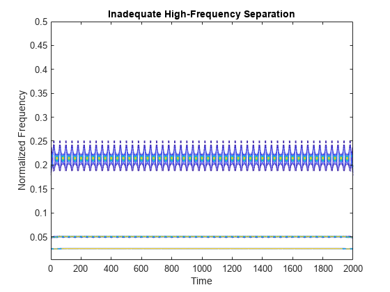
This example shows the separation needed between signal components to obtain usable results from the synchrosqueezed transform. The signal components are 0.025, 0.05, 0.20, and 0.225 cycles per sample. The high-frequency components, 0.20 and 0.225, do not have enough separation, so you cannot express the whole signal as a sum of well-separated IMTs.
Define the signal and plot the synchrosqueezed components.
t = 0:2000;
x1 = cos(2*pi*.025*t);
x2 = cos(2*pi*.05*t);
x3 = cos(2*pi*.20*t);
x4 = cos(2*pi*.225*t);
x =x1+x2+x3+x4;
[sst,f] = wsst(x);
contour(t,f,abs(sst))
xlabel("Time")
ylabel("Normalized Frequency")
title("Inadequate High-Frequency Separation")
Increase the separation of the high-frequency components, and then plot the synchrosqueezed components again.
x4 = cos(2*pi*.3*t);
x =x1+x2+x3+x4;
[sst,f] = wsst(x);
contour(t,f,abs(sst))
xlabel("Time")
ylabel("Normalized Frequency")
title("Adequate High-Frequency Separation")
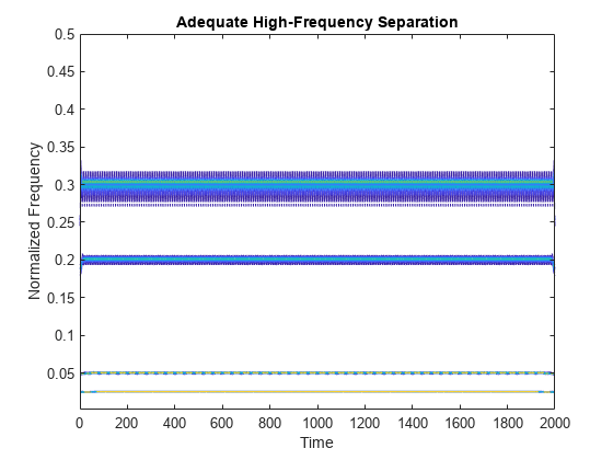
All the signal components are now well-separated IMTs and are separated enough to distinguish from each other. This signal is appropriate for use with the synchrosqueezing algorithm.
Region With Inadequate Separation
This example shows a signal with two linear chirps. A linear chirp is defined as
Its first derivative, , defines the instantaneous frequency line. Use the bump wavelet and its separation constant of 0.25. To determine the region where the two chirp signals with instantaneous frequencies of 0.4 and 0.1 cycles per sample are not separated enough, solve this equation:
and are the instantaneous frequency lines of the chirps.
t = 0:2000;
y1 = chirp(t,0.4,1000,0.25);
y2 = chirp(t,0.1,1000,0.25);
y = y1+y2;
wsst(y,'bump')
xlabel('Samples')
h1 = line([583 583], [0 0.5]);
h2 = line([1417 1417], [0 0.5]);
h1.Color='white';
h2.Color='white';
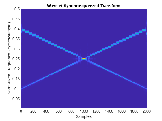
The vertical lines are the bounds of the region. They indicate that not enough separation occurs at sample 583 and sample 1417. In the region between the vertical lines, the signal does not consist of well-separated IMTs. In the regions outside the vertical lines, the signal has well-separated IMTs. You can obtain good results from the synchrosqueezed transform in these regions.
References
[1] Mallet, S. A Wavelet Tour of Signal Processing. San Diego, CA: Academic Press, 2008, p. 89.
[2] Daubechies, I., J. Lu, and H. T. Wu. "Synchrosqueezed Wavelet Transforms: an empirical mode decomposition-like tool." Applied and Computational Harmonic Analysis. Vol. 30(2), pp. 243–261.
[3] Thakur, G., E. Brevdo, N. S. Fučkar, and H. T. Wu. "The synchrosqueezing algorithm for time-varying spectral analysis: robustness properties and new paleoclimate applications." Signal Processing. Vol. 93, pp. 1079–1094.