uavCoverageSpace
R2026bDescription
The uavCoverageSpace object represents the coverage space as a set of
convex polygons to use with the uavCoveragePlanner to
perform coverage planning. Given a coverage area, the polygons form its configuration
space.
Creation
Syntax
Description
space = uavCoverageSpace creates an empty coverage space with
default properties.
space = uavCoverageSpace(Polygons=
creates a coverage space defined by one or more convex polygons as vertices
polygonVertices)polygonVertices, and sets the Polygons
property.
space = uavCoverageSpace(___,
sets properties using one or more name-value arguments. For example,
Name=Value)uavCoverageSpace(Overlap=0.5) sets the Overlap
property to 0.5.
Input Arguments
Properties
Object Functions
setCoveragePattern | Set sweep angle for polygon in coverage area |
show | Visualize 2D coverage space |
Examples
This example shows how to plan a coverage path that surveys the parking lots of the MathWorks Lakeside campus.
Get the geodetic coordinates for the MathWorks Lakeside campus, then create the limits for our map.
campusLocation = [42.3013 -71.375 0];
latlim = [campusLocation(1)-0.003 campusLocation(1)+0.003];
lonlim = [campusLocation(2)-0.003 campusLocation(2)+0.003];
Create a figure containing the map with the longitude and latitude limits.
fig = figure;
gx = geoaxes(fig,Basemap="satellite");
geolimits(latlim,lonlim)
Get the outline of the first parking lot in longitude and latitude coordinates. Then create the polygon by concatenating them.
parkingLot1Lat = [42.3028 42.30325 42.3027 42.3017 42.3019]';
parkingLot1Lon = [-71.37527 -71.37442 -71.3736 -71.37378 -71.375234]';
parkingLot1Poly = [parkingLot1Lat parkingLot1Lon];
Repeat the process for the second parking lot.
parkingLot2Lat = [42.30035 42.2999 42.2996 42.2999]';
parkingLot2Lon = [-71.3762 -71.3734 -71.37376 -71.37589]';
parkingLot2Poly = [parkingLot2Lat parkingLot2Lon];
Create the coverage space with both polygons, and specify these properties:
Waypoints coordinates format: Geodetic
Reference location: MathWorks Lakeside campus location
Reference height: 25 meters
Width of sensor footprint: 20 meters
parkingLotCoverage = uavCoverageSpace(Polygons={parkingLot1Poly,parkingLot2Poly},...
    UseLocalCoordinates=false,ReferenceLocation=campusLocation,...
    ReferenceHeight=25,UnitWidth=20);
Show the coverage space on the map.
show(parkingLotCoverage,Parent=gx);
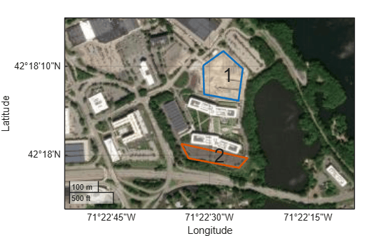
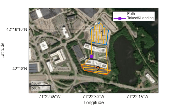
Set the sweep angle for polygons 1 and 2 to 85 and 5 degrees, respectively, to have paths that are parallel to the roads in the parking lots. Then create the coverage planner for that coverage space with the exhaustive solver algorithm.
setCoveragePattern(parkingLotCoverage,1,SweepAngle=85)
setCoveragePattern(parkingLotCoverage,2,SweepAngle=5)
lotPlanner = uavCoveragePlanner(parkingLotCoverage,Solver="Exhaustive");
Set the takeoff position to a location in the courtyard, then plan the coverage path.
takeoff = [42.30089 -71.3752, 0];
[plannedPath,solution] = plan(lotPlanner,takeoff);
hold on
geoplot(plannedPath(:,1),plannedPath(:,2),LineWidth=1.5);
geoplot(takeoff(1),takeoff(2),MarkerSize=25,Marker=".")
legend("","","Path","Takeoff/Landing")
hold off
This example shows how to plan a coverage path for a region in local coordinates and compares the results of using the exhaustive solver with the results of using the minimum traversal solver.
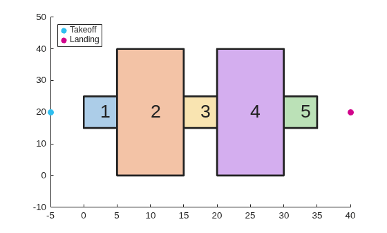
Define the vertices for a coverage space. This cross-shaped region creates multiple sub-regions that the solvers must visit in sequence.
area = [5 0; 5 15; 0 15; 0 25; 5 25; 5 40; 15 40; 15 25; 20 25; 20 40; ...
        30 40; 30 25; 35 25; 35 15; 30 15; 30 0; 20 0; 20 15; 15 15; 15 0];
Because the vertices define a concave polygon and the coverage planner requires convex polygons, decompose the polygon into convex polygons. Then, create a coverage space with the polygons from the decomposition.
polygons = coverageDecomposition(area);
centroids = cellfun(@(p) mean(p(:,1)),polygons);
[~,sortIdx] = sort(centroids);
polygons = polygons(sortIdx);
cs = uavCoverageSpace(Polygons=polygons);
Define the takeoff and landing positions. Then, show the coverage space and plot the takeoff and landing positions.
takeoff = [-5 20 0];
landing = [40 20 0];
show(cs);
exampleHelperPlotTakeoffLandingLegend(takeoff,landing)
Create a coverage planner with the exhaustive solver algorithm and another coverage planner with a minimum traversal solver algorithm.
The exhaustive solver iterates through all permutations of sweep options to minimize the connection distance between regions. This makes it better suited for smaller or separated regions. The minimum traversal solver uses a recursive traversal through a graph of adjacent polygons, making it faster and better suited for interconnected regions.
cpeExh = uavCoveragePlanner(cs,Solver="Exhaustive");
cpMin = uavCoveragePlanner(cs,Solver="MinTraversal");
Plan with both solver algorithms using the same takeoff and landing positions.
[wptsExh,solnExh] = plan(cpeExh,takeoff,landing);
[wptsMin,solnMin] = plan(cpMin,takeoff,landing);
Show the planned path for both the exhaustive and the minimum traversal algorithms.
figure
show(cs);
title("Exhaustive Solver Algorithm")
exampleHelperPlotTakeoffLandingLegend(takeoff,landing,wptsExh)
figure
show(cs);
title("Minimum Traversal Solver Algorithm")
exampleHelperPlotTakeoffLandingLegend(takeoff,landing,wptsMin)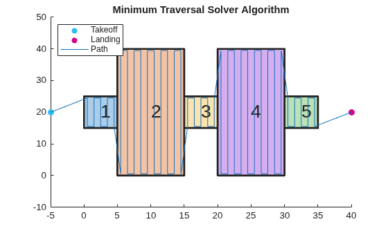
Compare the visiting sequences chosen by each solver. The exhaustive solver finds the globally optimal ordering by evaluating all permutations, while the minimum traversal solver prioritizes traversing adjacent polygons and flies to the nearest unvisited polygon when no adjacent ones remain.
disp("Exhaustive visiting sequence: " + mat2str(solnExh.VisitingSequence))Exhaustive visiting sequence: [1 2 4 5 3]
disp("MinTraversal visiting sequence: " + mat2str(solnMin.VisitingSequence))MinTraversal visiting sequence: [1 2 3 4 5]
Export the waypoints from the exhaustive solver to a .waypoints file with the reference frame set to north-east-down.
exportWaypointsPlan(cpeExh,solnExh,"coveragepath.waypoints",ReferenceFrame="NED")

