Train and Compare Classifiers Using Misclassification Costs in Classification Learner App
This example shows how to create and compare classifiers that use specified misclassification costs in the Classification Learner app. Specify the misclassification costs before training, and use the accuracy and total misclassification cost results to compare the trained models.
In the MATLAB® Command Window, load the
CreditRating_Historical.datfile into a table.openExample("CreditRating_Historical.dat")The Import Tool opens.
In the Imported Variable section on the Import tab, enter
creditratingin the Name box.In the Import section, click Import Selection and select Import Data.
Close the Import Tool. The predictor data consists of financial ratios and industry sector information for a list of corporate customers. The response variable consists of credit ratings assigned by a rating agency. Combine all the
Aratings into one rating. Do the same for theBandCratings, so that the response variable has three distinct ratings. Among the three ratings,Ais considered the best andCthe worst.Rating = categorical(creditrating.Rating); Rating = mergecats(Rating,["AAA","AA","A"],"A"); Rating = mergecats(Rating,["BBB","BB","B"],"B"); Rating = mergecats(Rating,["CCC","CC","C"],"C"); creditrating.Rating = Rating;
Assume these are the costs associated with misclassifying the credit ratings of customers.
Customer Predicted Rating ABCCustomer True Rating A$0 $100 $200 B$500 $0 $100 C$1000 $500 $0 For example, the cost of misclassifying a
Crating customer as anArating customer is $1000. The costs indicate that classifying a customer with bad credit as a customer with good credit is more costly than classifying a customer with good credit as a customer with bad credit.Create a matrix variable that contains the misclassification costs. Create another variable that specifies the class names and their order in the matrix variable.
ClassificationCosts = [0 100 200; 500 0 100; 1000 500 0];
ClassNames = categorical(["A","B","C"]);
Tip
Alternatively, you can specify misclassification costs directly inside the Classification Learner app. See Specify Misclassification Costs for more information.
Open Classification Learner using the
creditratingtable and theRatingvariable as the response.classificationLearner(creditrating,"Rating")To accept the default settings in the New Session from Arguments dialog box, click Start Session.
Specify the misclassification costs. On the Learn tab, in the Options section, click Costs. The app opens a dialog box showing the default misclassification costs.
In the dialog box, click Import from Workspace.

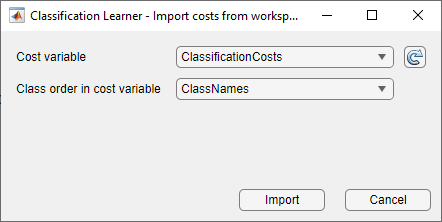
In the import dialog box, select
ClassificationCostsas the cost variable andClassNamesas the class order in the cost variable. Click Import.
The app updates the values in the misclassification costs dialog box. Click Save and Apply to save your changes. The new misclassification costs are applied to the existing draft model in the Models pane and will be applied to new draft models that you create using the gallery in the Models section of the Learn tab.

Train fine, medium, and coarse trees simultaneously. The Models pane already contains a fine tree model. Add medium and coarse tree models to the list of draft models. On the Learn tab, in the Models section, click the arrow to open the gallery. In the Decision Trees group, click Medium Tree. The app creates a draft medium tree and adds it to the Models pane. Reopen the model gallery and click Coarse Tree in the Decision Trees group. The app creates a draft coarse tree and adds it to the Models pane.
In the Train section, click Train All and select Train All. The app trains the three tree models.
Note
If you have Parallel Computing Toolbox™, then the Use Parallel button is selected by default. After you click Train All and select Train All or Train Selected, the app opens a parallel pool of workers. During this time, you cannot interact with the software. After the pool opens, you can continue to interact with the app while models train in parallel.
If you do not have Parallel Computing Toolbox, then the Use Background Training check box in the Train All menu is selected by default. After you select an option to train models, the app opens a background pool. After the pool opens, you can continue to interact with the app while models train in the background.

Note
Validation introduces some randomness into the results. Your model validation results can vary from the results shown in this example.
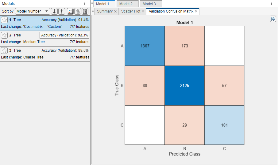
In the Models pane, each model has a validation accuracy score that indicates the percentage of correctly predicted responses. The app highlights the highest Accuracy (Validation) score by outlining it in a box.
Click a model to view the results, which are displayed in the Summary tab. To open this tab, right-click the model and select Summary.
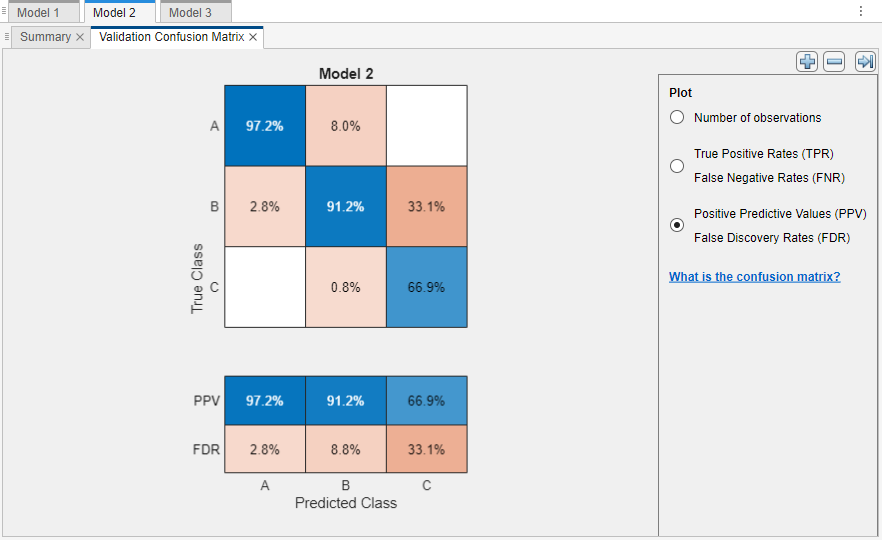
Inspect the accuracy of the predictions in each class. On the Learn tab, in the Plots and Results section, click the arrow to open the gallery, and then click Confusion Matrix (Validation) in the Validation Results group. The app displays a matrix of true class and predicted class results for the selected model (in this case, for the medium tree).

You can also plot results per predicted class to investigate false discovery rates. Under Plot, select the Positive Predictive Values (PPV) False Discovery Rates (FDR) option.
In the confusion matrix for the medium tree, the entries below the diagonal have small percentage values. These values indicate that the model tries to avoid assigning a credit rating that is higher than the true rating for a customer.

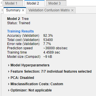
Compare the total misclassification costs of the tree models. To inspect the total misclassification cost of a model, select the model in the Models pane, and then view the Training Results section of the Summary tab. For example, the medium tree has these results.

Alternatively, you can sort the models based on the total misclassification cost. In the Models pane, open the Sort by list and select
Total Cost (Validation).In general, choose a model that has high accuracy and low total misclassification cost. In this example, the medium tree has the highest validation accuracy value and the lowest total misclassification cost of the three models.
You can perform feature selection and transformation or tune your model just as you do in the workflow without misclassification costs. However, always check the total misclassification cost of your model when assessing its performance. For information on how to find misclassification costs in the exported model and exported code, see Misclassification Costs in Exported Model and Generated Code.