Main Content

auc

Area under ROC curve or precision-recall curve

Since R2024b

Description

a = auc(rocObj) returns the area under the ROC (receiver operating characteristic) curve.

a = auc(rocObj,type) returns the area under the ROC curve when type is "roc", and returns the area under the precision-recall curve when type is "pr".

example

[a,lower,upper] = auc(___) additionally returns the lower and upper confidence bounds on a using any of the input argument combinations in the previous syntaxes.

example

Examples

collapse all

Fit a tree and a tree ensemble to data with unbalanced classes. Unbalanced data is most suited to the precision-recall curve.

Read the sample file CreditRating_Historical.dat into a table. The predictor data consists of financial ratios and industry sector information for a list of corporate customers. The response variable consists of credit ratings assigned by a rating agency. Preview the first few rows of the data set.

creditrating = readtable("CreditRating_Historical.dat");
head(creditrating)
     ID      WC_TA     RE_TA     EBIT_TA    MVE_BVTD    S_TA     Industry    Rating 
    _____    ______    ______    _______    ________    _____    ________    _______

    62394     0.013     0.104     0.036      0.447      0.142        3       {'BB' }
    48608     0.232     0.335     0.062      1.969      0.281        8       {'A'  }
    42444     0.311     0.367     0.074      1.935      0.366        1       {'A'  }
    48631     0.194     0.263     0.062      1.017      0.228        4       {'BBB'}
    43768     0.121     0.413     0.057      3.647      0.466       12       {'AAA'}
    39255    -0.117    -0.799      0.01      0.179      0.082        4       {'CCC'}
    62236     0.087     0.158     0.049      0.816      0.324        2       {'BBB'}
    39354     0.005     0.181     0.034      2.597      0.388        7       {'AA' }

Because each value in the ID variable is a unique customer ID, that is, length(unique(creditrating.ID)) is equal to the number of observations in creditrating, the ID variable is a poor predictor. Remove the ID variable from the table, and convert the Industry variable to a categorical variable.

creditrating = removevars(creditrating,"ID");
creditrating.Industry = categorical(creditrating.Industry);

Count the number of observations with each credit rating.

classCounts = groupcounts(creditrating,"Rating")
classCounts=7×3 table
    Rating     GroupCount    Percent
    _______    __________    _______

    {'A'  }        575       14.624 
    {'AA' }        385       9.7915 
    {'AAA'}        580       14.751 
    {'B'  }        320       8.1384 
    {'BB' }        927       23.576 
    {'BBB'}       1015       25.814 
    {'CCC'}        130       3.3062 

The data has unbalanced classes.

Partition the data into training and test sets using cvpartition.

rng("default") % For reproducibility of the partition
c = cvpartition(creditrating.Rating,"Holdout",0.5);
trainingIndices = training(c); % Indices for the training set
testIndices = test(c); % Indices for the test set
creditTrain = creditrating(trainingIndices,:);
creditTest = creditrating(testIndices,:);

Train a tree and a tree ensemble using the training data. Compute the positive predictive value (PPV), or precision, for each class using the test data.

tree = fitctree(creditTrain,"Rating");
ens = fitcensemble(creditTrain,"Rating");
treeROC = rocmetrics(tree,creditTest,"Rating",AdditionalMetrics="prec");
ensROC = rocmetrics(ens,creditTest,"Rating",AdditionalMetrics="prec");

Compare the precision-recall AUC results for the tree and ensemble.

treePRAUC = auc(treeROC,"pr")
treePRAUC = 1×7

    0.6539    0.6502    0.9304    0.3713    0.5920    0.6464    0.7015

ensPRAUC = auc(ensROC,"pr")
ensPRAUC = 1×7

    0.8074    0.8238    0.9886    0.6156    0.7453    0.8134    0.8647

The ensemble has a better set of precision-recall AUC values.

Find the AUC for a cross-validated quadratic discriminant model of the fisheriris data, and return the bounds on the statistics. By default, cross-validated classification models create confidence intervals, so lower and upper bounds are available in areaUnderCurve.

load fisheriris
rng default % For reproducibility
Mdl = fitcdiscr(meas,species,DiscrimType="quadratic",KFold=5);
rocObj = rocmetrics(Mdl);
[a,lower,upper] = auc(rocObj)
a = 1×3

    1.0000    0.9984    0.9984

lower = 1×3

    1.0000    0.9970    0.9970

upper = 1×3

    1.0000    0.9998    0.9998

For the Fisher iris data, the AUC values are all essentially equal to 1.

Input Arguments

collapse all

Object evaluating classification performance, specified as a rocmetrics object.

Type of AUC to compute, specified as "roc" for the area under the ROC curve, or "pr" for the area under the precision-recall curve.

Data Types: char | string

Output Arguments

collapse all

Area under the curve, returned as a double or single vector, where each element of a represents the area for a class.

Lower confidence bounds on AUC, returned as a double or single vector, where each element of lower represents the confidence bound for a class. The object must be created with confidence intervals for the function to return this output.

Upper confidence bounds on AUC, returned as a double or single vector, where each element of upper represents the confidence bound for a class. The object must be created with confidence intervals for the function to return this output.

Algorithms

For an ROC curve, auc calculates the area under the curve by trapezoidal integration using the trapz function. For a precision-recall curve, auc calculates the area under the curve using the trapz function, and then adds the area of the rectangle (if any) that is formed by the leftmost point on the curve and the point (0,0). For example,

load ionosphere
rng default % For reproducibility of the partition
c = cvpartition(Y,Holdout=0.25);
trainingIndices = training(c); % Indices for the training set
testIndices = test(c); % Indices for the test set
XTrain = X(trainingIndices,:);
YTrain = Y(trainingIndices);
XTest = X(testIndices,:);
YTest = Y(testIndices);
Mdl = fitcsvm(XTrain,YTrain);
rocObj = rocmetrics(Mdl,XTest,YTest,AdditionalMetrics="ppv");
r = plot(rocObj,XAxisMetric="tpr",...
    YAxisMetric="ppv",ClassNames="b"); % Plots the normal PR curve.
legend(Location="southeast")

Performance curve showing a gap between x = 0 and the leftmost point on the curve.

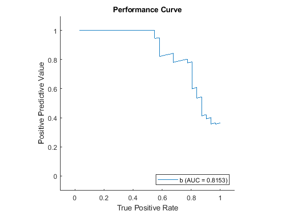
There is a gap between the leftmost point on the curve and the zero point of the True Positive Rate. Plot the rectangle that fills this gap, which represents the correction that auc adds to the returned AUC.

hold on
rectangle(Position=[0 0 r.XData(2) r.YData(2)],FaceColor=r.Color)
hold off

A rectangle fills the gap between the leftmost point on the curve and 0.

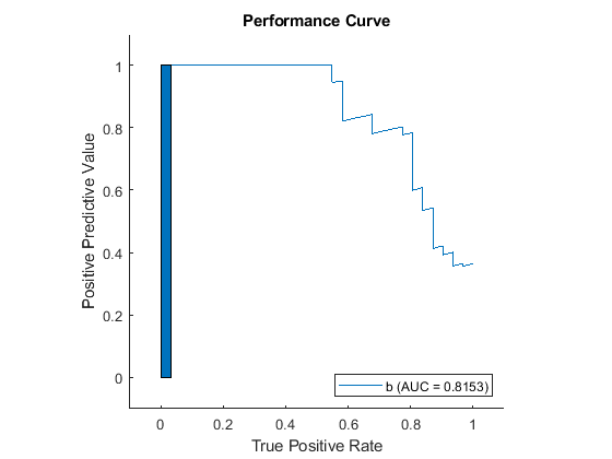
Technically, the rectangle is not part of the precision-recall curve. But to make comparisons easier across models (which can have different domains of definition), auc treats the area under the curve as extending all the way down to zero.

If you create a rocmetrics object with confidence intervals (as described on the reference page), the returned AUC lower and upper arguments use the same technique for computing confidence intervals as done for the original rocmetrics object, either bootstrapping or cross-validation.

Version History

Introduced in R2024b

See Also

| |