resume

Resume training of Gaussian kernel regression model

Syntax

UpdatedMdl = resume(Mdl,X,Y)

UpdatedMdl = resume(Mdl,Tbl,ResponseVarName)

UpdatedMdl = resume(Mdl,Tbl,Y)

UpdatedMdl = resume(___,Name,Value)

[UpdatedMdl,FitInfo] = resume(___)

Description

UpdatedMdl = resume(Mdl,X,Y) continues training with the same options used to train Mdl, including the training data (predictor data in X and response data in Y) and the feature expansion. The training starts at the current estimated parameters in Mdl. The function returns a new Gaussian kernel regression model UpdatedMdl.

UpdatedMdl = resume(Mdl,Tbl,ResponseVarName) continues training with the predictor data in Tbl and the true responses in Tbl.ResponseVarName.

UpdatedMdl = resume(Mdl,Tbl,Y) continues training with the predictor data in table Tbl and the true responses in Y.

UpdatedMdl = resume(___,Name,Value) specifies options using one or more name-value pair arguments in addition to any of the input argument combinations in previous syntaxes. For example, you can modify convergence control options, such as convergence tolerances and the maximum number of additional optimization iterations.

[UpdatedMdl,FitInfo] = resume(___) also returns the fit information in the structure array FitInfo.

Examples

Estimate Sample Loss and Resume Training

Resume training a Gaussian kernel regression model for more iterations to improve the regression loss.

Load the carbig data set.

load carbig

Specify the predictor variables (X) and the response variable (Y).

X = [Acceleration,Cylinders,Displacement,Horsepower,Weight];
Y = MPG;

Delete rows of X and Y where either array has NaN values. Removing rows with NaN values before passing data to fitrkernel can speed up training and reduce memory usage.

R = rmmissing([X Y]); % Data with missing entries removed
X = R(:,1:5); 
Y = R(:,end); 

Reserve 10% of the observations as a holdout sample. Extract the training and test indices from the partition definition.

rng(10)  % For reproducibility
N = length(Y);
cvp = cvpartition(N,'Holdout',0.1);
idxTrn = training(cvp); % Training set indices
idxTest = test(cvp);    % Test set indices

Train a kernel regression model. Standardize the training data, set the iteration limit to 5, and specify 'Verbose',1 to display diagnostic information.

Xtrain = X(idxTrn,:);
Ytrain = Y(idxTrn);

Mdl = fitrkernel(Xtrain,Ytrain,'Standardize',true, ...
    'IterationLimit',5,'Verbose',1)

|=================================================================================================================|
| Solver |  Pass  |   Iteration  |   Objective   |     Step      |    Gradient   |    Relative    |  sum(beta~=0) |
|        |        |              |               |               |   magnitude   | change in Beta |               |
|=================================================================================================================|
|  LBFGS |      1 |            0 |  5.691016e+00 |  0.000000e+00 |  5.852758e-02 |                |             0 |
|  LBFGS |      1 |            1 |  5.086537e+00 |  8.000000e+00 |  5.220869e-02 |   9.846711e-02 |           256 |
|  LBFGS |      1 |            2 |  3.862301e+00 |  5.000000e-01 |  3.796034e-01 |   5.998808e-01 |           256 |
|  LBFGS |      1 |            3 |  3.460613e+00 |  1.000000e+00 |  3.257790e-01 |   1.615091e-01 |           256 |
|  LBFGS |      1 |            4 |  3.136228e+00 |  1.000000e+00 |  2.832861e-02 |   8.006254e-02 |           256 |
|  LBFGS |      1 |            5 |  3.063978e+00 |  1.000000e+00 |  1.475038e-02 |   3.314455e-02 |           256 |
|=================================================================================================================|

Mdl = 
  RegressionKernel
              ResponseName: 'Y'
                   Learner: 'svm'
    NumExpansionDimensions: 256
               KernelScale: 1
                    Lambda: 0.0028
             BoxConstraint: 1
                   Epsilon: 0.8617


  Properties, Methods

Mdl is a RegressionKernel model.

Estimate the epsilon-insensitive error for the test set.

Xtest = X(idxTest,:);
Ytest = Y(idxTest);

L = loss(Mdl,Xtest,Ytest,'LossFun','epsiloninsensitive')

L = 
2.0674

Continue training the model by using resume. This function continues training with the same options used for training Mdl.

UpdatedMdl = resume(Mdl,Xtrain,Ytrain);

|=================================================================================================================|
| Solver |  Pass  |   Iteration  |   Objective   |     Step      |    Gradient   |    Relative    |  sum(beta~=0) |
|        |        |              |               |               |   magnitude   | change in Beta |               |
|=================================================================================================================|
|  LBFGS |      1 |            0 |  3.063978e+00 |  0.000000e+00 |  1.475038e-02 |                |           256 |
|  LBFGS |      1 |            1 |  3.007822e+00 |  8.000000e+00 |  1.391637e-02 |   2.603966e-02 |           256 |
|  LBFGS |      1 |            2 |  2.817171e+00 |  5.000000e-01 |  5.949008e-02 |   1.918084e-01 |           256 |
|  LBFGS |      1 |            3 |  2.807294e+00 |  2.500000e-01 |  6.798867e-02 |   2.973097e-02 |           256 |
|  LBFGS |      1 |            4 |  2.791060e+00 |  1.000000e+00 |  2.549575e-02 |   1.639328e-02 |           256 |
|  LBFGS |      1 |            5 |  2.767821e+00 |  1.000000e+00 |  6.154419e-03 |   2.468903e-02 |           256 |
|  LBFGS |      1 |            6 |  2.738163e+00 |  1.000000e+00 |  5.949008e-02 |   9.476263e-02 |           256 |
|  LBFGS |      1 |            7 |  2.719146e+00 |  1.000000e+00 |  1.699717e-02 |   1.849972e-02 |           256 |
|  LBFGS |      1 |            8 |  2.705941e+00 |  1.000000e+00 |  3.116147e-02 |   4.152590e-02 |           256 |
|  LBFGS |      1 |            9 |  2.701162e+00 |  1.000000e+00 |  5.665722e-03 |   9.401466e-03 |           256 |
|  LBFGS |      1 |           10 |  2.695341e+00 |  5.000000e-01 |  3.116147e-02 |   4.968046e-02 |           256 |
|  LBFGS |      1 |           11 |  2.691277e+00 |  1.000000e+00 |  8.498584e-03 |   1.017446e-02 |           256 |
|  LBFGS |      1 |           12 |  2.689972e+00 |  1.000000e+00 |  1.983003e-02 |   9.938921e-03 |           256 |
|  LBFGS |      1 |           13 |  2.688979e+00 |  1.000000e+00 |  1.416431e-02 |   6.606316e-03 |           256 |
|  LBFGS |      1 |           14 |  2.687787e+00 |  1.000000e+00 |  1.621956e-03 |   7.089542e-03 |           256 |
|  LBFGS |      1 |           15 |  2.686539e+00 |  1.000000e+00 |  1.699717e-02 |   1.169701e-02 |           256 |
|  LBFGS |      1 |           16 |  2.685356e+00 |  1.000000e+00 |  1.133144e-02 |   1.069310e-02 |           256 |
|  LBFGS |      1 |           17 |  2.685021e+00 |  5.000000e-01 |  1.133144e-02 |   2.104248e-02 |           256 |
|  LBFGS |      1 |           18 |  2.684002e+00 |  1.000000e+00 |  2.832861e-03 |   6.175231e-03 |           256 |
|  LBFGS |      1 |           19 |  2.683507e+00 |  1.000000e+00 |  5.665722e-03 |   3.724026e-03 |           256 |
|  LBFGS |      1 |           20 |  2.683343e+00 |  5.000000e-01 |  5.665722e-03 |   9.549119e-03 |           256 |
|=================================================================================================================|
| Solver |  Pass  |   Iteration  |   Objective   |     Step      |    Gradient   |    Relative    |  sum(beta~=0) |
|        |        |              |               |               |   magnitude   | change in Beta |               |
|=================================================================================================================|
|  LBFGS |      1 |           21 |  2.682897e+00 |  1.000000e+00 |  5.665722e-03 |   7.172867e-03 |           256 |
|  LBFGS |      1 |           22 |  2.682682e+00 |  1.000000e+00 |  2.832861e-03 |   2.587726e-03 |           256 |
|  LBFGS |      1 |           23 |  2.682485e+00 |  1.000000e+00 |  2.832861e-03 |   2.953648e-03 |           256 |
|  LBFGS |      1 |           24 |  2.682326e+00 |  1.000000e+00 |  2.832861e-03 |   7.777294e-03 |           256 |
|  LBFGS |      1 |           25 |  2.681914e+00 |  1.000000e+00 |  2.832861e-03 |   2.778555e-03 |           256 |
|  LBFGS |      1 |           26 |  2.681867e+00 |  5.000000e-01 |  1.031085e-03 |   3.638352e-03 |           256 |
|  LBFGS |      1 |           27 |  2.681725e+00 |  1.000000e+00 |  5.665722e-03 |   1.515199e-03 |           256 |
|  LBFGS |      1 |           28 |  2.681692e+00 |  5.000000e-01 |  1.314940e-03 |   1.850055e-03 |           256 |
|  LBFGS |      1 |           29 |  2.681625e+00 |  1.000000e+00 |  2.832861e-03 |   1.456903e-03 |           256 |
|  LBFGS |      1 |           30 |  2.681594e+00 |  5.000000e-01 |  2.832861e-03 |   8.704875e-04 |           256 |
|  LBFGS |      1 |           31 |  2.681581e+00 |  5.000000e-01 |  8.498584e-03 |   3.934768e-04 |           256 |
|  LBFGS |      1 |           32 |  2.681579e+00 |  1.000000e+00 |  8.498584e-03 |   1.847866e-03 |           256 |
|  LBFGS |      1 |           33 |  2.681553e+00 |  1.000000e+00 |  9.857038e-04 |   6.509825e-04 |           256 |
|  LBFGS |      1 |           34 |  2.681541e+00 |  5.000000e-01 |  8.498584e-03 |   6.635528e-04 |           256 |
|  LBFGS |      1 |           35 |  2.681499e+00 |  1.000000e+00 |  5.665722e-03 |   6.194735e-04 |           256 |
|  LBFGS |      1 |           36 |  2.681493e+00 |  5.000000e-01 |  1.133144e-02 |   1.617763e-03 |           256 |
|  LBFGS |      1 |           37 |  2.681473e+00 |  1.000000e+00 |  9.869233e-04 |   8.418484e-04 |           256 |
|  LBFGS |      1 |           38 |  2.681469e+00 |  1.000000e+00 |  5.665722e-03 |   1.069722e-03 |           256 |
|  LBFGS |      1 |           39 |  2.681432e+00 |  1.000000e+00 |  2.832861e-03 |   8.501930e-04 |           256 |
|  LBFGS |      1 |           40 |  2.681423e+00 |  2.500000e-01 |  1.133144e-02 |   9.543716e-04 |           256 |
|=================================================================================================================|
| Solver |  Pass  |   Iteration  |   Objective   |     Step      |    Gradient   |    Relative    |  sum(beta~=0) |
|        |        |              |               |               |   magnitude   | change in Beta |               |
|=================================================================================================================|
|  LBFGS |      1 |           41 |  2.681416e+00 |  1.000000e+00 |  2.832861e-03 |   8.763251e-04 |           256 |
|  LBFGS |      1 |           42 |  2.681413e+00 |  5.000000e-01 |  2.832861e-03 |   4.101888e-04 |           256 |
|  LBFGS |      1 |           43 |  2.681403e+00 |  1.000000e+00 |  5.665722e-03 |   2.713209e-04 |           256 |
|  LBFGS |      1 |           44 |  2.681392e+00 |  1.000000e+00 |  2.832861e-03 |   2.115241e-04 |           256 |
|  LBFGS |      1 |           45 |  2.681383e+00 |  1.000000e+00 |  2.832861e-03 |   2.872858e-04 |           256 |
|  LBFGS |      1 |           46 |  2.681374e+00 |  1.000000e+00 |  8.498584e-03 |   5.771001e-04 |           256 |
|  LBFGS |      1 |           47 |  2.681353e+00 |  1.000000e+00 |  2.832861e-03 |   3.160871e-04 |           256 |
|  LBFGS |      1 |           48 |  2.681334e+00 |  5.000000e-01 |  8.498584e-03 |   1.045502e-03 |           256 |
|  LBFGS |      1 |           49 |  2.681314e+00 |  1.000000e+00 |  7.878714e-04 |   1.505118e-03 |           256 |
|  LBFGS |      1 |           50 |  2.681306e+00 |  1.000000e+00 |  2.832861e-03 |   4.756894e-04 |           256 |
|  LBFGS |      1 |           51 |  2.681301e+00 |  1.000000e+00 |  1.133144e-02 |   3.664873e-04 |           256 |
|  LBFGS |      1 |           52 |  2.681288e+00 |  1.000000e+00 |  2.832861e-03 |   1.449821e-04 |           256 |
|  LBFGS |      1 |           53 |  2.681287e+00 |  2.500000e-01 |  1.699717e-02 |   2.357176e-04 |           256 |
|  LBFGS |      1 |           54 |  2.681282e+00 |  1.000000e+00 |  5.665722e-03 |   2.046663e-04 |           256 |
|  LBFGS |      1 |           55 |  2.681278e+00 |  1.000000e+00 |  2.832861e-03 |   2.546349e-04 |           256 |
|  LBFGS |      1 |           56 |  2.681276e+00 |  2.500000e-01 |  1.307940e-03 |   1.966786e-04 |           256 |
|  LBFGS |      1 |           57 |  2.681274e+00 |  5.000000e-01 |  1.416431e-02 |   1.005310e-04 |           256 |
|  LBFGS |      1 |           58 |  2.681271e+00 |  5.000000e-01 |  1.118892e-03 |   1.147324e-04 |           256 |
|  LBFGS |      1 |           59 |  2.681269e+00 |  1.000000e+00 |  2.832861e-03 |   1.332914e-04 |           256 |
|  LBFGS |      1 |           60 |  2.681268e+00 |  2.500000e-01 |  1.132045e-03 |   5.441369e-05 |           256 |
|=================================================================================================================|

Estimate the epsilon-insensitive error for the test set using the updated model.

UpdatedL = loss(UpdatedMdl,Xtest,Ytest,'LossFun','epsiloninsensitive')

UpdatedL = 
1.8933

The regression error decreases by a factor of about 0.08 after resume updates the regression model with more iterations.

Resume Training with Modified Convergence Control Training Options

Load the carbig data set.

load carbig

Specify the predictor variables (X) and the response variable (Y).

X = [Acceleration,Cylinders,Displacement,Horsepower,Weight];
Y = MPG;

Delete rows of X and Y where either array has NaN values. Removing rows with NaN values before passing data to fitrkernel can speed up training and reduce memory usage.

R = rmmissing([X Y]); % Data with missing entries removed
X = R(:,1:5); 
Y = R(:,end); 

Reserve 10% of the observations as a holdout sample. Extract the training and test indices from the partition definition.

rng(10)  % For reproducibility
N = length(Y);
cvp = cvpartition(N,'Holdout',0.1);
idxTrn = training(cvp); % Training set indices
idxTest = test(cvp);    % Test set indices

Train a kernel regression model with relaxed convergence control training options by using the name-value arguments 'BetaTolerance' and 'GradientTolerance'. Standardize the training data, and specify 'Verbose',1 to display diagnostic information.

Xtrain = X(idxTrn,:);
Ytrain = Y(idxTrn);

[Mdl,FitInfo] = fitrkernel(Xtrain,Ytrain,'Standardize',true,'Verbose',1, ...
    'BetaTolerance',2e-2,'GradientTolerance',2e-2);

|=================================================================================================================|
| Solver |  Pass  |   Iteration  |   Objective   |     Step      |    Gradient   |    Relative    |  sum(beta~=0) |
|        |        |              |               |               |   magnitude   | change in Beta |               |
|=================================================================================================================|
|  LBFGS |      1 |            0 |  5.691016e+00 |  0.000000e+00 |  5.852758e-02 |                |             0 |
|  LBFGS |      1 |            1 |  5.086537e+00 |  8.000000e+00 |  5.220869e-02 |   9.846711e-02 |           256 |
|  LBFGS |      1 |            2 |  3.862301e+00 |  5.000000e-01 |  3.796034e-01 |   5.998808e-01 |           256 |
|  LBFGS |      1 |            3 |  3.460613e+00 |  1.000000e+00 |  3.257790e-01 |   1.615091e-01 |           256 |
|  LBFGS |      1 |            4 |  3.136228e+00 |  1.000000e+00 |  2.832861e-02 |   8.006254e-02 |           256 |
|  LBFGS |      1 |            5 |  3.063978e+00 |  1.000000e+00 |  1.475038e-02 |   3.314455e-02 |           256 |
|=================================================================================================================|

Mdl is a RegressionKernel model.

Estimate the epsilon-insensitive error for the test set.

Xtest = X(idxTest,:);
Ytest = Y(idxTest);

L = loss(Mdl,Xtest,Ytest,'LossFun','epsiloninsensitive')

L = 
2.0674

Continue training the model by using resume with modified convergence control options.

[UpdatedMdl,UpdatedFitInfo] = resume(Mdl,Xtrain,Ytrain, ...
    'BetaTolerance',2e-3,'GradientTolerance',2e-3);

|=================================================================================================================|
| Solver |  Pass  |   Iteration  |   Objective   |     Step      |    Gradient   |    Relative    |  sum(beta~=0) |
|        |        |              |               |               |   magnitude   | change in Beta |               |
|=================================================================================================================|
|  LBFGS |      1 |            0 |  3.063978e+00 |  0.000000e+00 |  1.475038e-02 |                |           256 |
|  LBFGS |      1 |            1 |  3.007822e+00 |  8.000000e+00 |  1.391637e-02 |   2.603966e-02 |           256 |
|  LBFGS |      1 |            2 |  2.817171e+00 |  5.000000e-01 |  5.949008e-02 |   1.918084e-01 |           256 |
|  LBFGS |      1 |            3 |  2.807294e+00 |  2.500000e-01 |  6.798867e-02 |   2.973097e-02 |           256 |
|  LBFGS |      1 |            4 |  2.791060e+00 |  1.000000e+00 |  2.549575e-02 |   1.639328e-02 |           256 |
|  LBFGS |      1 |            5 |  2.767821e+00 |  1.000000e+00 |  6.154419e-03 |   2.468903e-02 |           256 |
|  LBFGS |      1 |            6 |  2.738163e+00 |  1.000000e+00 |  5.949008e-02 |   9.476263e-02 |           256 |
|  LBFGS |      1 |            7 |  2.719146e+00 |  1.000000e+00 |  1.699717e-02 |   1.849972e-02 |           256 |
|  LBFGS |      1 |            8 |  2.705941e+00 |  1.000000e+00 |  3.116147e-02 |   4.152590e-02 |           256 |
|  LBFGS |      1 |            9 |  2.701162e+00 |  1.000000e+00 |  5.665722e-03 |   9.401466e-03 |           256 |
|  LBFGS |      1 |           10 |  2.695341e+00 |  5.000000e-01 |  3.116147e-02 |   4.968046e-02 |           256 |
|  LBFGS |      1 |           11 |  2.691277e+00 |  1.000000e+00 |  8.498584e-03 |   1.017446e-02 |           256 |
|  LBFGS |      1 |           12 |  2.689972e+00 |  1.000000e+00 |  1.983003e-02 |   9.938921e-03 |           256 |
|  LBFGS |      1 |           13 |  2.688979e+00 |  1.000000e+00 |  1.416431e-02 |   6.606316e-03 |           256 |
|  LBFGS |      1 |           14 |  2.687787e+00 |  1.000000e+00 |  1.621956e-03 |   7.089542e-03 |           256 |
|=================================================================================================================|

Estimate the epsilon-insensitive error for the test set using the updated model.

UpdatedL = loss(UpdatedMdl,Xtest,Ytest,'LossFun','epsiloninsensitive')

UpdatedL = 
1.8891

The regression error decreases after resume updates the regression model with smaller convergence tolerances.

Display the outputs FitInfo and UpdatedFitInfo.

FitInfo

FitInfo = struct with fields:
                  Solver: 'LBFGS-fast'
            LossFunction: 'epsiloninsensitive'
                  Lambda: 0.0028
           BetaTolerance: 0.0200
       GradientTolerance: 0.0200
          ObjectiveValue: 3.0640
       GradientMagnitude: 0.0148
    RelativeChangeInBeta: 0.0331
                 FitTime: 0.0395
                 History: [1×1 struct]

UpdatedFitInfo

UpdatedFitInfo = struct with fields:
                  Solver: 'LBFGS-fast'
            LossFunction: 'epsiloninsensitive'
                  Lambda: 0.0028
           BetaTolerance: 0.0020
       GradientTolerance: 0.0020
          ObjectiveValue: 2.6878
       GradientMagnitude: 0.0016
    RelativeChangeInBeta: 0.0071
                 FitTime: 0.0534
                 History: [1×1 struct]

Both trainings terminate because the software satisfies the absolute gradient tolerance.

Plot the gradient magnitude versus the number of iterations by using UpdatedFitInfo.History.GradientMagnitude. Note that the History field of UpdatedFitInfo includes the information in the History field of FitInfo.

semilogy(UpdatedFitInfo.History.GradientMagnitude,'o-')
ax = gca;
ax.XTick = 1:21;
ax.XTickLabel = UpdatedFitInfo.History.IterationNumber;
grid on
xlabel('Number of Iterations')
ylabel('Gradient Magnitude')

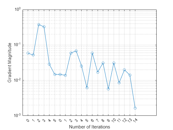
The first training terminates after five iterations because the gradient magnitude becomes less than 2e-2. The second training terminates after 14 iterations because the gradient magnitude becomes less than 2e-3.

Input Arguments

Mdl — Kernel regression model

RegressionKernel model object

Kernel regression model, specified as a RegressionKernel model object. You can create a RegressionKernel model object using fitrkernel.

X — Predictor data used to train Mdl

n-by-p numeric matrix

Predictor data used to train Mdl, specified as an n-by-p numeric matrix, where n is the number of observations and p is the number of predictors.

Data Types: single | double

Y — Response data used to train Mdl

numeric vector

Response data used to train Mdl, specified as a numeric vector.

Data Types: double | single

Tbl — Sample data used to train Mdl

table

Sample data used to train Mdl, specified as a table. Each row of Tbl corresponds to one observation, and each column corresponds to one predictor variable. Optionally, Tbl can contain additional columns for the response variable and observation weights. Tbl must contain all of the predictors used to train Mdl. Multicolumn variables and cell arrays other than cell arrays of character vectors are not allowed.

If you trained Mdl using sample data contained in a table, then the input data for resume must also be in a table.

ResponseVarName — Name of response variable used to train Mdl

name of variable in Tbl

Name of the response variable used to train Mdl, specified as the name of a variable in Tbl. The ResponseVarName value must match the name Mdl.ResponseName.

Data Types: char | string

Note

resume should run only on the same training data and observation weights (Weights) used to train Mdl. The resume function uses the same training options, such as feature expansion, used to train Mdl.

Name-Value Arguments

Specify optional pairs of arguments as Name1=Value1,...,NameN=ValueN, where Name is the argument name and Value is the corresponding value. Name-value arguments must appear after other arguments, but the order of the pairs does not matter.

Before R2021a, use commas to separate each name and value, and enclose Name in quotes.

Example: UpdatedMdl = resume(Mdl,X,Y,'BetaTolerance',1e-3) resumes training with the same options used to train Mdl, except the relative tolerance on the linear coefficients and the bias term.

Weights — Observation weights used to train Mdl

numeric vector | name of variable in Tbl

Observation weights used to train Mdl, specified as the comma-separated pair consisting of 'Weights' and a numeric vector or the name of a variable in Tbl.

• If Weights is a numeric vector, then the size of Weights must be equal to the number of rows in X or Tbl.

• If Weights is the name of a variable in Tbl, you must specify Weights as a character vector or string scalar. For example, if the weights are stored as Tbl.W, then specify Weights as 'W'. Otherwise, the software treats all columns of Tbl, including Tbl.W, as predictors.

If you supply the observation weights, resume normalizes Weights to sum to 1.

Data Types: double | single | char | string

BetaTolerance — Relative tolerance on linear coefficients and bias term

BetaTolerance value used to train Mdl (default) | nonnegative scalar

Relative tolerance on the linear coefficients and the bias term (intercept), specified as a nonnegative scalar.

Let $$B_t=\left[{\beta }_t{}^{\prime }{b}_t\right]$$, that is, the vector of the coefficients and the bias term at optimization iteration t. If $${\Vert \frac{B_t-B_{t-1}}{B_t}\Vert }_2<\text{BetaTolerance}$$, then optimization terminates.

If you also specify GradientTolerance, then optimization terminates when the software satisfies either stopping criterion.

By default, the value is the same BetaTolerance value used to train Mdl.

Example: 'BetaTolerance',1e-6

Data Types: single | double

GradientTolerance — Absolute gradient tolerance

GradientTolerance value used to train Mdl (default) | nonnegative scalar

Absolute gradient tolerance, specified as a nonnegative scalar.

Let $$\nabla {ℒ}_t$$ be the gradient vector of the objective function with respect to the coefficients and bias term at optimization iteration t. If $${\Vert \nabla {ℒ}_t\Vert }_{\infty }=\max \left|\nabla {ℒ}_t\right|<\text{GradientTolerance}$$, then optimization terminates.

If you also specify BetaTolerance, then optimization terminates when the software satisfies either stopping criterion.

By default, the value is the same GradientTolerance value used to train Mdl.

Example: 'GradientTolerance',1e-5

Data Types: single | double

IterationLimit — Maximum number of additional optimization iterations

positive integer

Maximum number of additional optimization iterations, specified as the comma-separated pair consisting of 'IterationLimit' and a positive integer.

The default value is 1000 if the transformed data fits in memory (Mdl.ModelParameters.BlockSize), which you specify by using the 'BlockSize' name-value pair argument when training Mdl with fitrkernel. Otherwise, the default value is 100.

Note that the default value is not the value used to train Mdl.

Example: 'IterationLimit',500

Data Types: single | double

Output Arguments

UpdatedMdl — Updated kernel regression model

RegressionKernel model object

Updated kernel regression model, returned as a RegressionKernel model object.

FitInfo — Optimization details

structure array

Optimization details, returned as a structure array including fields described in this table. The fields contain final values or name-value pair argument specifications.

Field	Description
Solver	Objective function minimization technique: 'LBFGS-fast', 'LBFGS-blockwise', or 'LBFGS-tall'. For details, see the Algorithms section of fitrkernel.
LossFunction	Loss function. Either mean squared error (MSE) or epsilon-insensitive, depending on the type of linear regression model. See Learner of fitrkernel.
Lambda	Regularization term strength. See Lambda of fitrkernel.
BetaTolerance	Relative tolerance on the linear coefficients and the bias term. See BetaTolerance.
GradientTolerance	Absolute gradient tolerance. See GradientTolerance.
ObjectiveValue	Value of the objective function when optimization terminates. The regression loss plus the regularization term compose the objective function.
GradientMagnitude	Infinite norm of the gradient vector of the objective function when optimization terminates. See GradientTolerance.
RelativeChangeInBeta	Relative changes in the linear coefficients and the bias term when optimization terminates. See BetaTolerance.
FitTime	Elapsed, wall-clock time (in seconds) required to fit the model to the data.
History	History of optimization information. This field also includes the optimization information from training Mdl. This field is empty ([]) if you specify 'Verbose',0 when training Mdl. For details, see Verbose and the Algorithms section of fitrkernel.

To access fields, use dot notation. For example, to access the vector of objective function values for each iteration, enter FitInfo.ObjectiveValue in the Command Window.

Examine the information provided by FitInfo to assess whether convergence is satisfactory.

More About

Random Feature Expansion

Random feature expansion, such as Random Kitchen Sinks [1] or Fastfood [2], is a scheme to approximate Gaussian kernels of the kernel regression algorithm for big data in a computationally efficient way. Random feature expansion is more practical for big data applications that have large training sets, but can also be applied to smaller data sets that fit in memory.

After mapping the predictor data into a high-dimensional space, the kernel regression algorithm searches for an optimal function that deviates from each response data point (y_i) by values no greater than the epsilon margin (ε).

Some regression problems cannot be described adequately using a linear model. In such cases, obtain a nonlinear regression model by replacing the dot product x₁x₂′ with a nonlinear kernel function $$G(x_1,x_2)=\langle \phi (x_1),\phi (x_2)\rangle$$, where x_i is the ith observation (row vector) and φ(x_i) is a transformation that maps x_i to a high-dimensional space (called the “kernel trick”). However, evaluating G(x₁,x₂), the Gram matrix, for each pair of observations is computationally expensive for a large data set (large n).

The random feature expansion scheme finds a random transformation so that its dot product approximates the Gaussian kernel. That is,

$$G(x_1,x_2)=\langle \phi (x_1),\phi (x_2)\rangle \approx T(x_1)T(x_2)\text{'},$$

where T(x) maps x in $${ℝ}^p$$ to a high-dimensional space ($${ℝ}^m$$). The Random Kitchen Sinks [1] scheme uses the random transformation

$$T(x)=m^{-1/2}\exp \left(iZx\text{'}\right)\text{'},$$

where $$Z\in {ℝ}^{m\times p}$$ is a sample drawn from $$N\left(0,{\sigma }^{-2}\right)$$ and σ is a kernel scale. This scheme requires O(mp) computation and storage. The Fastfood [2] scheme introduces another random basis V instead of Z using Hadamard matrices combined with Gaussian scaling matrices. This random basis reduces computation cost to O(mlogp) and reduces storage to O(m).

You can specify values for m and σ, using the NumExpansionDimensions and KernelScale name-value pair arguments of fitrkernel, respectively.

The fitrkernel function uses the Fastfood scheme for random feature expansion and uses linear regression to train a Gaussian kernel regression model. Unlike solvers in the fitrsvm function, which require computation of the n-by-n Gram matrix, the solver in fitrkernel only needs to form a matrix of size n-by-m, with m typically much less than n for big data.

Extended Capabilities

Tall Arrays

Calculate with arrays that have more rows than fit in memory.

The resume function supports tall arrays with the following usage notes and limitations:

• resume does not support tall table data.

• The default value for the 'IterationLimit' name-value pair argument is relaxed to 20 when you work with tall arrays.

• resume uses a block-wise strategy. For details, see the Algorithms section of fitrkernel.

For more information, see Tall Arrays.

GPU Arrays

Accelerate code by running on a graphics processing unit (GPU) using Parallel Computing Toolbox™. (since R2025a)

This function fully supports GPU arrays. For more information, see Run MATLAB Functions on a GPU (Parallel Computing Toolbox).

Version History

Introduced in R2018a

R2025a: Specify GPU arrays (requires Parallel Computing Toolbox)

resume fully supports GPU arrays.