Multiple Comparisons
Analysis of variance (ANOVA) techniques test whether a set of group means (treatment effects) are equal or not. Rejection of the null hypothesis leads to the conclusion that not all group means are the same. This result, however, does not provide further information on which group means are different.
Performing a series of t-tests to determine which pairs of means are significantly different is not recommended. When you perform multiple t-tests, the probability that the means appear significant, and significant difference results might be due to large number of tests. These t-tests use the data from the same sample, hence they are not independent. This fact makes it more difficult to quantify the level of significance for multiple tests.
Suppose that in a single t-test, the probability that the null hypothesis (H0) is rejected when it is actually true is a small value, say 0.05. Suppose also that you conduct six independent t-tests. If the significance level for each test is 0.05, then the probability that the tests correctly fail to reject H0, when H0 is true for each case, is (0.95)6 = 0.735. And the probability that one of the tests incorrectly rejects the null hypothesis is 1 – 0.735 = 0.265, which is much higher than 0.05.
To compensate for multiple tests, you can use multiple comparison procedures. The
multcompare function performs multiple
pairwise comparisons of the group means, or treatment effects. The options are Tukey’s
honestly significant difference criterion (default option), the Bonferroni method,
Scheffé’s procedure, Fisher’s least significant differences (LSD) method, and Dunn &
Sidák’s approach to t-test. The function also supports Dunnett's
test, which performs multiple comparisons against a control group.
To perform multiple comparisons of group means, provide the structure
stats as an input for multcompare. You can
obtain stats from one of the following functions:
kruskalwallis— Nonparametric method for one-way layoutfriedman— Nonparametric method for two-way layout
For multiple comparison procedure options for repeated measures, see multcompare (RepeatedMeasuresModel).
Multiple Comparisons Using One-Way ANOVA
Load the sample data.
load carsmallMPG represents the miles per gallon for each car, and Cylinders represents the number of cylinders in each car, either 4, 6, or 8 cylinders.
Test if the mean miles per gallon (mpg) is different across cars that have different numbers of cylinders. Also compute the statistics needed for multiple comparison tests.
[p,~,stats] = anova1(MPG,Cylinders,"off");
p
p = 4.4902e-24
The small p-value of about 0 is a strong indication that mean miles per gallon is significantly different across cars with different numbers of cylinders.
Perform a multiple comparison test, using the Bonferroni method, to determine which numbers of cylinders make a difference in the performance of the cars.
[results,means,~,gnames] = multcompare(stats,"CriticalValueType","bonferroni");

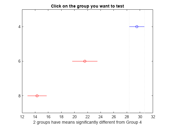
In the figure the blue bar represents the group of cars with 4 cylinders. The red bars represent the other groups. None of the red comparison intervals for the mean mpg of cars overlap, which means that the mean mpg is significantly different for cars having 4, 6, or 8 cylinders.
Display the multiple comparison results and the corresponding group names in a table.
tbl = array2table([results,means],"VariableNames", ...
    ["Group A","Group B","Lower Limit","A-B","Upper Limit","P-value","Mean","Standard Error"]);
tbl.("Group A")=gnames(tbl.("Group A"));
tbl.("Group B")=gnames(tbl.("Group B"))
tbl=3×8 table
    Group A    Group B    Lower Limit     A-B      Upper Limit     P-value       Mean     Standard Error
    _______    _______    ___________    ______    ___________    __________    ______    ______________

     {'4'}      {'6'}       4.8605       7.9418      11.023       3.3159e-08     29.53       0.63634
     {'4'}      {'8'}       12.613       15.234      17.855       2.7661e-24    21.588        1.0913
     {'6'}      {'8'}        3.894       7.2919       10.69        3.172e-06    14.296       0.86596
The first two columns of the results matrix show which groups are compared. For example, the first row compares the cars with 4 and 6 cylinders. The fourth column shows the mean mpg difference for the compared groups. The third and fifth columns show the lower and upper limits for a 95% confidence interval for the difference in the group means. The last column shows the p-values for the tests. All p-values are nearly zero, which indicates that the mean mpg for all groups differ across all groups.
The first column of the means matrix has the mean mpg estimates for each group of cars. The second column contains the standard errors of the estimates.
Multiple Comparisons for Three-Way ANOVA
Load the sample data.
y = [52.7 57.5 45.9 44.5 53.0 57.0 45.9 44.0]';
g1 = [1 2 1 2 1 2 1 2];
g2 = ["hi" "hi" "lo" "lo" "hi" "hi" "lo" "lo"];
g3 = ["may" "may" "may" "may" "june" "june" "june" "june"];
y is the response vector and g1, g2, and g3 are the grouping variables (factors). Each factor has two levels, and every observation in y is identified by a combination of factor levels. For example, observation y(1) is associated with level 1 of factor g1, level hi of factor g2, and level may of factor g3. Similarly, observation y(6) is associated with level 2 of factor g1, level hi of factor g2, and level june of factor g3.
Test if the response is the same for all factor levels. Also compute the statistics required for multiple comparison tests.
[~,~,stats] = anovan(y,{g1 g2 g3},"Model","interaction", ...
    "Varnames",["g1","g2","g3"]);
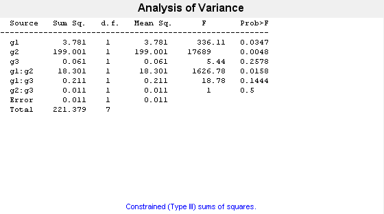
The p-value of 0.2578 indicates that the mean responses for levels may and june of factor g3 are not significantly different. The p-value of 0.0347 indicates that the mean responses for levels 1 and 2 of factor g1 are significantly different. Similarly, the p-value of 0.0048 indicates that the mean responses for levels hi and lo of factor g2 are significantly different.
Perform a multiple comparison test to find out which groups of factors g1 and g2 are significantly different.
[results,~,~,gnames] = multcompare(stats,"Dimension",[1 2]);
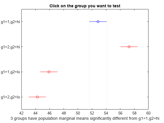
You can test the other groups by clicking on the corresponding comparison interval for the group. The bar you click on turns to blue. The bars for the groups that are significantly different are red. The bars for the groups that are not significantly different are gray. For example, if you click on the comparison interval for the combination of level 1 of g1 and level lo of g2, the comparison interval for the combination of level 2 of g1 and level lo of g2 overlaps, and is therefore gray. Conversely, the other comparison intervals are red, indicating significant difference.
Display the multiple comparison results and the corresponding group names in a table.
tbl = array2table(results,"VariableNames", ...
    ["Group A","Group B","Lower Limit","A-B","Upper Limit","P-value"]);
tbl.("Group A")=gnames(tbl.("Group A"));
tbl.("Group B")=gnames(tbl.("Group B"))
tbl=6×6 table
       Group A           Group B        Lower Limit     A-B     Upper Limit     P-value
    ______________    ______________    ___________    _____    ___________    _________

    {'g1=1,g2=hi'}    {'g1=2,g2=hi'}      -6.8604       -4.4      -1.9396       0.027249
    {'g1=1,g2=hi'}    {'g1=1,g2=lo'}       4.4896       6.95       9.4104       0.016983
    {'g1=1,g2=hi'}    {'g1=2,g2=lo'}       6.1396        8.6        11.06       0.013586
    {'g1=2,g2=hi'}    {'g1=1,g2=lo'}       8.8896      11.35        13.81       0.010114
    {'g1=2,g2=hi'}    {'g1=2,g2=lo'}        10.54         13        15.46      0.0087375
    {'g1=1,g2=lo'}    {'g1=2,g2=lo'}      -0.8104       1.65       4.1104        0.07375
The multcompare function compares the combinations of groups (levels) of the two grouping variables, g1 and g2. For example, the first row of the matrix shows that the combination of level 1 of g1 and level hi of g2 has the same mean response values as the combination of level 2 of g1 and level hi of g2. The p-value corresponding to this test is 0.0272, which indicates that the mean responses are significantly different. You can also see this result in the figure. The blue bar shows the comparison interval for the mean response for the combination of level 1 of g1 and level hi of g2. The red bars are the comparison intervals for the mean response for other group combinations. None of the red bars overlap with the blue bar, which means the mean response for the combination of level 1 of g1 and level hi of g2 is significantly different from the mean response for other group combinations.
Multiple Comparison Procedures
Specify the multiple comparison procedure by setting the CriticalValueType name-value
argument to one of the values in this table.
| Value | Description |
|---|---|
"lsd" | Fisher's least significant difference procedure |
"dunnett" | Dunnett's test |
"tukey-kramer" or "hsd" (default) | Tukey’s honestly significant difference procedure |
"dunn-sidak" | Dunn & Sidák’s approach |
"bonferroni" | Bonferroni method |
"scheffe" | Scheffé’s procedure |
The table lists the critical value types in order of conservativeness, from least to most conservative. Each test provides a different level of protection against the multiple comparison problem.
"lsd"does not provide any protection."dunnett"provides protection for comparisons against a control group."tukey-kramer","dunn-sidak", and"bonferroni"provide protection for pairwise comparisons."scheffe"provides protection for pairwise comparisons and comparisons of all linear combinations of the estimates.
The multcompare function
examines different sets of null hypotheses (H0) and
alternative hypotheses (H1) depending on the type of
critical value specified by the CriticalValueType name-value argument.
Dunnett's test (
CriticalValueTypeis"dunnett") performs multiple comparisons against a control group. Therefore, the null and alternative hypotheses for a comparison against the control group arewhere mi and m0 are estimates for group i and the control group, respectively. The function examines H0 and H1 multiple times for all noncontrol groups.
For the other tests,
multcompareperforms multiple pairwise comparisons for all distinct pairs of groups. The null and alternative hypotheses of a pairwise comparison between group i and j are
Fisher's Least Significant Difference Procedure
Specify CriticalValueType as "lsd" to
use the least significance difference procedure. This test uses the test
statistic
It rejects H0:mi = mj if
Fisher suggests a protection against multiple comparisons by performing LSD only when the null hypothesis H0: m1 = m2 = ... = mk is rejected by ANOVA F-test. Even in this case, LSD might not reject any of the individual hypotheses. It is also possible that ANOVA does not reject H0, even when there are differences between some group means. This behavior occurs because the equality of the remaining group means can cause the F-test statistic to be nonsignificant. Without any condition, LSD does not provide any protection against the multiple comparison problem.
Dunnett's Test
Specify CriticalValueType as "dunnett"
to use Dunnett's test. This test is for multiple comparisons against a control
group. You can specify the control group by using the ControlGroup name-value argument. The test statistic for
Dunnett's test depends on the source of the group means. If you examine the
group means from a one-way ANOVA, the test statistic is
The test rejects H0
: mi =
m0 if |ti| <
d. The multcompare function finds
d by solving the equation
where p is the number of noncontrol groups, and F(⋯|C,ν) is the cumulative distribution function (cdf) of a multivariate t distribution with the correlation matrix C and degrees of freedom ν.
Finding d can be slow for multiway
(n-way) ANOVA if n is large. To speed up
the computation, you can use an approximation method ([5]) by specifying the
Approximate name-value argument as true
(default for multiway ANOVA). The approximate method involves randomness. If you
want to reproduce the results, set the random seed by using the rng function before calling
multcompare.
Tukey’s Honestly Significant Difference Procedure
Specify CriticalValueType as
"Tukey-Kramer" or "hsd" to use Tukey’s
honestly significant difference procedure. The test is based on studentized
range distribution. Reject
H0:mi
= mj if
where is the upper 100*(1 – α)th percentile of the studentized range distribution with parameter k and N – k degrees of freedom. k is the number of groups (treatments or marginal means) and N is the total number of observations.
Tukey’s honestly significant difference procedure is optimal for balanced one-way ANOVA and similar procedures with equal sample sizes. It has been proven to be conservative for one-way ANOVA with different sample sizes. According to the unproven Tukey-Kramer conjecture, it is also accurate for problems where the quantities being compared are correlated, as in analysis of covariance with unbalanced covariate values.
Dunn & Sidák’s Approach
Specify CriticalValueType as
"dunn-sidak" to use Dunn & Sidák’s approach. It uses
critical values from the t-distribution, after an adjustment
for multiple comparisons that was proposed by Dunn and proved accurate by Sidák.
This test rejects
H0:mi
= mj if
where
and k is the number of groups. This procedure is similar to, but less conservative than, the Bonferroni procedure.
Bonferroni Method
Specify CriticalValueType as
"bonferroni" to use the Bonferroni method. This method
uses critical values from Student’s t-distribution after an
adjustment to compensate for multiple comparisons. The test rejects
H0:mi
= mj at the significance level, where k is the number
of groups if
where N is the total number of observations and k is the number of groups (marginal means). This procedure is conservative, but usually less so than the Scheffé procedure.
Scheffé’s Procedure
Specify CriticalValueType as "scheffe"
to use Scheffé’s procedure. The critical values are derived from the
F distribution. The test rejects
H0:mi
= mj if
This procedure provides a simultaneous confidence level for comparisons of all linear combinations of the means. It is conservative for comparisons of simple differences of pairs.
References
[1] Milliken G. A. and D. E. Johnson. Analysis of Messy Data. Volume I: Designed Experiments. Boca Raton, FL: Chapman & Hall/CRC Press, 1992.
[2] Neter J., M. H. Kutner, C. J. Nachtsheim, W. Wasserman. 4th ed. Applied Linear Statistical Models.Irwin Press, 1996.
[3] Hochberg, Y., and A. C. Tamhane. Multiple Comparison Procedures. Hoboken, NJ: John Wiley & Sons, 1987.
See Also
multcompare | anova1 | anova2 | anovan | aoctool | kruskalwallis | friedman