Model-Specific Anomaly Detection
Statistics and Machine Learning Toolbox™ provides model-specific anomaly detection features that you can apply after training a classification, regression, or clustering model. For example, you can detect anomalies by using these object functions:
Proximity matrix —
outlierMeasurefor random forest (CompactTreeBagger)Mahalanobis distance —
mahalfor discriminant analysis classifier (ClassificationDiscriminant) andmahalfor Gaussian mixture model (gmdistribution)Unconditional probability density —
logpfor discriminant analysis classifier (ClassificationDiscriminant),logpfor naive Bayes classifier (ClassificationNaiveBayes), andlogpfor naive Bayes classifier for incremental learning (incrementalClassificationNaiveBayes)
For details, see the function reference pages.
Detect Outliers After Training Random Forest
Train a random forest classifier by using the TreeBagger function, and detect outliers in the training data by using the object function outlierMeasure.
Train Random Forest Classifier
Load the ionosphere data set, which contains radar return qualities (Y) and predictor data (X) for 34 variables. Radar returns are either of good quality ('g') or bad quality ('b').
load ionosphereTrain a random forest classifier. Store the out-of-bag information for predictor importance estimation.
rng("default") % For reproducibility
Mdl_TB = TreeBagger(100,X,Y,Method="classification", ...
    OOBPredictorImportance="on");
Mdl_TB is a TreeBagger model object for classification. TreeBagger stores predictor importance estimates in the property OOBPermutedPredictorDeltaError.
Detect Outliers Using Proximity
Detect outliers in the training data by using the outlierMeasure function. The function computes outlier measures based on the average squared proximity between one observation and the other observations in the trained random forest.
CMdl_TB = compact(Mdl_TB);
s_proximity = outlierMeasure(CMdl_TB,X,Labels=Y);
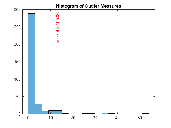
A high value of the outlier measure indicates that the observation is an outlier. Find the threshold corresponding to the 95th percentile and identify outliers by using the isoutlier function.
[TF,~,U] = isoutlier(s_proximity,Percentiles=[0 95]);
Plot a histogram of the outlier measures. Create a vertical line at the outlier threshold.
histogram(s_proximity)
xline(U,"r-",join(["Threshold =" U]))
title("Histogram of Outlier Measures")
Visualize observation values using the two most important features selected by the predictor importance estimates in the property OOBPermutedPredictorDeltaError.
[~,idx] = sort(Mdl_TB.OOBPermutedPredictorDeltaError,'descend');
TF_c = categorical(TF,[0 1],["Normal Points" "Anomalies"]);
gscatter(X(:,idx(1)),X(:,idx(2)),TF_c,"kr",".x",[],"on", ...
    Mdl_TB.PredictorNames(idx(1)),Mdl_TB.PredictorNames(idx(2)))

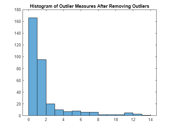
Train the classifier again without outliers, and plot the histogram of the outlier measures.
Mdl_TB = TreeBagger(100,X(~TF,:),Y(~TF),Method="classification");
s_proximity = outlierMeasure(CMdl_TB,X(~TF,:),Labels=Y(~TF));
histogram(s_proximity)
title("Histogram of Outlier Measures After Removing Outliers")
Detect Outliers After Training Discriminant Analysis Classifier
Train a discriminant analysis model by using the fitcdiscr function, and detect outliers in the training data by using the object functions logp and mahal.
Train Discriminant Analysis Model
Load Fisher's iris data set. The matrix meas contains flower measurements for 150 different flowers. The variable species lists the species for each flower.
load fisheririsTrain a discriminant analysis model using the entire data set.
Mdl = fitcdiscr(meas,species,PredictorNames= ...
    ["Sepal Length" "Sepal Width" "Petal Length" "Petal Width"]);
Mdl is a ClassificationDiscriminant model.
Detect Outliers Using Log Unconditional Probability Density
Compute the log unconditional probability densities of the training data.
s_logp = logp(Mdl,meas);
A low density value indicates that the corresponding observation is an outlier.
Determine the lower density threshold for outliers by using the isoutlier function.
[~,L_logp] = isoutlier(s_logp);
Identify outliers by using the threshold.
TF_logp = s_logp < L_logp;
Plot a histogram of the density values. Create a vertical line at the outlier threshold.
figure
histogram(s_logp)
xline(L_logp,"r-",join(["Threshold =" L_logp]))
title("Histogram of Log Unconditional Probability Densities ")

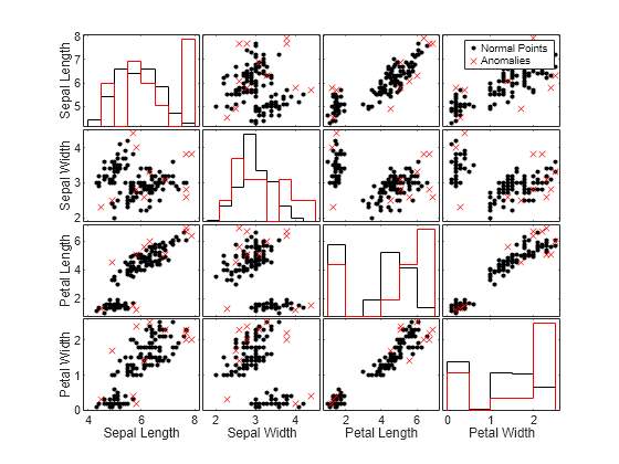
To compare observation values between normal points and anomalies, create a matrix of grouped histograms and grouped scatter plots for each combination of variables by using the gplotmatrix function.
TF_logp_c = categorical(TF_logp,[0 1],["Normal Points" "Anomalies"]);
gplotmatrix(meas,[],TF_logp_c,"kr",".x",[],[],[],Mdl.PredictorNames)
Detect Outliers Using Mahalanobis Distance
Find the squared Mahalanobis distances from the training data to the class means of true labels.
s_mahal = mahal(Mdl,meas,ClassLabels=species);
A large distance value indicates that the corresponding observation is an outlier.
Determine the threshold corresponding to the 95th percentile and identify outliers by using the isoutlier function.
[TF_mahal,~,U_mahal] = isoutlier(s_mahal,Percentiles=[0 95]);
Plot a histogram of the distances. Create a vertical line at the outlier threshold.
figure
histogram(s_mahal)
xline(U_mahal,"-r",join(["Threshold =" U_mahal]))
title("Histogram of Mahalanobis Distances")

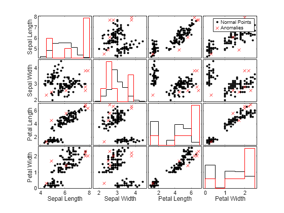
Compare the observation values between normal points and anomalies by using the gplotmatrix function.
TF_mahal_c = categorical(TF_mahal,[0 1],["Normal Points" "Anomalies"]);
gplotmatrix(meas,[],TF_mahal_c,"kr",".x",[],[],[],Mdl.PredictorNames)
See Also
outlierMeasure | mahal
(ClassificationDiscriminant) | mahal
(gmdistribution) | logp
(ClassificationDiscriminant) | logp
(ClassificationNaiveBayes) | logp
(incrementalClassificationNaiveBayes) | isoutlier