isanomaly

Find anomalies in data using one-class support vector machine (SVM) for incremental learning

Since R2023b

Syntax

tf = isanomaly(Mdl,Tbl)

tf = isanomaly(Mdl,X)

tf = isanomaly(___,ScoreThreshold=scoreThreshold)

[tf,scores] = isanomaly(___)

Description

tf = isanomaly(Mdl,Tbl) finds anomalies in the table Tbl using the incrementalOneClassSVM object Mdl and returns the logical array tf, whose elements are true when an anomaly is detected in the corresponding row of Tbl. You must use this syntax if you create Mdl by passing a table to incrementalOneClassSVM or the incrementalLearner function of OneClassSVM.

tf = isanomaly(Mdl,X) finds anomalies in the matrix X. You must use this syntax if you create Mdl by passing a matrix to incrementalOneClassSVM or the incrementalLearner function of OneClassSVM.

tf = isanomaly(___,ScoreThreshold=scoreThreshold) specifies the threshold for the anomaly score using any of the input argument combinations in the previous syntaxes. isanomaly detects observations with scores above scoreThreshold as anomalies.

[tf,scores] = isanomaly(___) also returns an anomaly score in the range (–inf,inf) for each observation in Tbl or X. A negative score value with large magnitude indicates a normal observation, and a large positive value indicates an anomaly.

Examples

Incrementally Train One-Class SVM Model on Shingled Data

Train a one-class SVM model on a simulated noisy periodic shingled time series containing no anomalies by using ocsvm. Convert the trained model to an incremental learner object, and incrementally fit the time series and detect anomalies.

Create Simulated Data Stream

Create a simulated data stream of observations representing a noisy sinusoid signal.

rng(0,"twister"); % For reproducibility
period = 100;
n = 5001+period;
sigma = 0.04;
a = linspace(1,n,n)';
b = sin(2*pi*(a-1)/period)+sigma*randn(n,1);

Introduce an anomalous region into the data stream. Plot the data stream portion which contains the anomalous region, and circle the anomalous data points.

c = 2*(sin(2*pi*(a-35)/period)+sigma*randn(n,1));

b(2150:2170) = c(2150:2170);
scatter(a,b,".")
xlim([1900,2200])
xlabel("Observation")
hold on
scatter(a(2150:2170),b(2150:2170),"r")
hold off

Convert the single-featured data set b into a multi-featured data set by shingling [1] with a shingle size equal to the period of the signal. The $$i$$th shingled observation is a vector of $$k$$ features with values $$b_i$$, $$b_{i+1}$$, ..., $$b_{i+k-1}$$, where $$k$$ is the shingle size.

X = [];
shingleSize = period;
for i = 1:n-shingleSize
    X = [X;b(i:i+shingleSize-1)'];
end

Train Model and Perform Incremental Anomaly Detection

Fit a one-class SVM model to the first 1000 shingled observations, specifying a contamination fraction of zero. Convert it to an incrementalOneClassSVM model object.

Mdl = ocsvm(X(1:1000,:),ContaminationFraction=0);
IncrementalMdl = incrementalLearner(Mdl);

To simulate a data stream, process the full shingled data set in chunks of 100 observations at a time. At each iteration:

• Process 100 observations.

• Calculate scores and detect anomalies using the isanomaly function.

• Store anomIdx, the indices of shingled observations marked as anomalies.

• If the chunk contains fewer than three anomalies, fit and update the previous incremental model.

n = numel(X(:,1));
numObsPerChunk = 100;
nchunk = floor(n/numObsPerChunk);
anomIdx = [];
allscores = [];

% Incremental fitting
rng(0,"twister"); % For reproducibility
for j = 1:nchunk
    ibegin = min(n,numObsPerChunk*(j-1) + 1);
    iend = min(n,numObsPerChunk*j);
    idx = ibegin:iend;
    [isanom,scores] = isanomaly(IncrementalMdl,X(idx,:));
    allscores = [allscores;scores];
    anomIdx = [anomIdx;find(isanom)+ibegin-1];
    if (sum(isanom) < 3)
        IncrementalMdl = fit(IncrementalMdl,X(idx,:));
    end
end

Analyze Incremental Model During Training

At each iteration, the software calculates a score value for each observation in the data chunk. A negative score value with large magnitude indicates a normal observation, and a large positive value indicates an anomaly. Plot the anomaly score for the observations in the vicinity of the anomaly. Circle the scores of shingles that the software returns as anomalous.

figure
scatter(a(1:5000),allscores,".")
hold on
scatter(a(anomIdx),allscores(anomIdx),20,"or")
xlim([1900,2200])
xlabel("Shingle")
ylabel("Score")
hold off

Because the introduced anomalous region begins at observation 2150, and the shingle size is 100, shingle 2051 is the first one to show a high anomaly score. Some shingles between 2050 and 2170 have scores lying just below the anomaly score threshold due to the noise in the sinusoidal signal. The shingle size affects the performance of the model by defining how many subsequent consecutive data points in the original time series the software uses to calculate the anomaly score for each shingle.

Plot the unshingled data and highlight the introduced anomalous region. Circle the observation number of the first element in each shingle that the software returned as anomalous.

figure
xlim([1900,2200])
ylim([-1.5 2])
rectangle(Position=[2150 -1.5 20 3.5],FaceColor=[0.9 0.9 0.9], ...
    EdgeColor=[0.9 0.9 0.9])
hold on
scatter(a,b,".")
scatter(a(anomIdx),b(anomIdx),20,"or")
xlabel("Observation")
hold off

Perform Incremental Anomaly Detection Using a Score Threshold Buffer

Perform incremental anomaly detection using a score threshold buffer on a simulated noisy periodic shingled time series containing anomalies.

Create Simulated Data Stream

Create a simulated data stream of observations representing a noisy sinusoid signal.

rng(0,"twister"); % For reproducibility
period = 100;
n = 5000;
sigma = 0.18;
a = linspace(1,n,n)';
X1 = sin(2*pi*a/period)+sigma*randn(n,1);
X2 = sin(2*pi*a/period/3)+sigma*randn(n,1);

Introduce an anomalous region into the data stream.

c = 5*sin(2*pi*(a-35)/period+sigma*randn(n,1));
X1(4051:4070) = c(4051:4070);
X2(4051:4070) = c(4051:4070);
X = [X1 X2];

Create Incremental One-Class SVM Model

Create an incrementalOneClassSVM model object. Specify a score warm-up period of 1000 observations.

scoreWarmupPeriod = 1000;
IncrementalMdl = incrementalOneClassSVM(ScoreWarmupPeriod=scoreWarmupPeriod);

Fit Incremental Model and Detect Anomalies

To simulate a data stream, process the full data set in chunks of 100 observations at a time. At each iteration:

• Process 100 observations.

• If the incremental model is warm, calculate scores and detect anomalies using the isanomaly function.

• Store allscores, the scores of the observations.

• Store anomIdx, the indices of observations detected as anomalies.

• If the chunk contains fewer than three anomalies, fit and update the previous incremental model.

numObsPerChunk = 100;
nchunk = floor(n/numObsPerChunk);
anomIdx = [];
allscores = [];
isanom = [];

% Incremental fitting
for j = 1:nchunk
    ibegin = min(n,numObsPerChunk*(j-1) + 1);
    iend = min(n,numObsPerChunk*j);
    idx = ibegin:iend;
    if (IncrementalMdl.IsWarm)
        [isanom,scores] = isanomaly(IncrementalMdl,X(idx,:));
        allscores = [allscores;scores];
        anomIdx = [anomIdx;find(isanom)+ibegin-1];
    end    
    if (sum(isanom) < 3)
        IncrementalMdl = fit(IncrementalMdl,X(idx,:));
    end
end

Plot the scores for observations after the warm-up period. Circle the detected anomalies and indicate the introduced anomalous observations with an x marker.

scatter(a(scoreWarmupPeriod+1:end),allscores(1:end),".")
xlabel("Observation")
ylabel("Score")
hold on
scatter(a(4051:4070), ...
    allscores(4051-scoreWarmupPeriod:4070-scoreWarmupPeriod),90,"x")
scatter(a(anomIdx),allscores(anomIdx-scoreWarmupPeriod),20,"or")
hold off

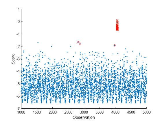
The software detects all of the observations in the introduced anomalous region as anomalies. However, the software also detects several other observations as anomalies due to the noisy sinusoid signal.

Detect Anomalies Using a Score Threshold Buffer

Repeat the incremental anomaly detection procedure with a new incremental one-class SVM model. Specify a score warm-up period of 1000 observations. Only observations with scores above ScoreThreshold + thresholdBuffer are detected as anomalies. Specify thresholdBuffer = 1.

thresholdBuffer = 1;
scoreWarmupPeriod = 1000;
IncrementalMdl = incrementalOneClassSVM(ScoreWarmupPeriod=scoreWarmupPeriod);
numObsPerChunk = 100;
nchunk = floor(n/numObsPerChunk);
anomIdx = [];
allscores = [];
isanom = [];

% Incremental fitting
for j = 1:nchunk
    ibegin = min(n,numObsPerChunk*(j-1) + 1);
    iend = min(n,numObsPerChunk*j);
    idx = ibegin:iend;
    if (IncrementalMdl.IsWarm)
        [isanom,scores] = isanomaly(IncrementalMdl,X(idx,:), ...
            ScoreThreshold=IncrementalMdl.ScoreThreshold+thresholdBuffer);
        allscores = [allscores;scores];
        anomIdx = [anomIdx;find(isanom)+ibegin-1];
    end    
    if (sum(isanom) < 3)
        IncrementalMdl = fit(IncrementalMdl,X(idx,:));
    end
end

Plot the scores for observations after the warm-up period. The scores are different from those in the previous model due to the stochastic behavior of the one-class SVM training algorithm, which incorporates random feature expansion. Circle the detected anomalies and indicate the introduced anomalous observations with an x marker.

scatter(a(scoreWarmupPeriod+1:end),allscores(1:end),".")
xlabel("Observation")
ylabel("Score")
hold on
scatter(a(4051:4070), ...
    allscores(4051-scoreWarmupPeriod:4070-scoreWarmupPeriod),90,"x")
scatter(a(anomIdx),allscores(anomIdx-scoreWarmupPeriod),20,"or")
hold off

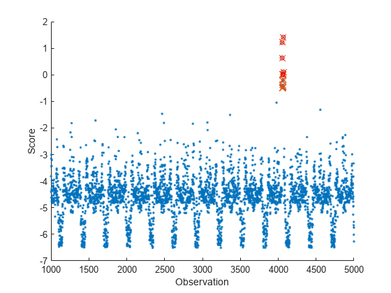
The software detects only the observations in the introduced anomalous region as anomalies.

Input Arguments

Mdl — Trained one-class SVM model

incrementalOneClassSVM object

Trained one-class SVM model, specified as an incrementalOneClassSVM model object.

Tbl — Predictor data

table

Predictor data, specified as a table. Each row of Tbl corresponds to one observation, and each column corresponds to one predictor variable. Multicolumn variables and cell arrays other than cell arrays of character vectors are not allowed.

If you train Mdl using a table, then you must provide predictor data by using Tbl, not X. All predictor variables in Tbl must have the same variable names and data types as those in the training data. However, the column order in Tbl does not need to correspond to the column order of the training data.

Note

Incremental learning functions support only numeric input predictor data. You must prepare an encoded version of categorical data to use incremental learning functions. Use dummyvar to convert each categorical variable to a dummy variable. For more details, see Dummy Variables.

Data Types: table

X — Predictor data

numeric matrix

Predictor data, specified as a numeric matrix. Each row of X corresponds to one observation, and each column corresponds to one predictor variable.

If you train Mdl using a matrix, then you must provide predictor data by using X, not Tbl. The variables that make up the columns of X must have the same order as the columns in the training data.

Note

Incremental learning functions support only numeric input predictor data. You must prepare an encoded version of categorical data to use incremental learning functions. Use dummyvar to convert each categorical variable to a numeric matrix of dummy variables. Then, concatenate all dummy variable matrices and any other numeric predictors, in the same way that the training function encodes categorical data. For more details, see Dummy Variables.

Data Types: single | double

scoreThreshold — Threshold for anomaly score

Mdl.ScoreThreshold (default) | numeric scalar in the range (–Inf,Inf)

Threshold for the anomaly score, specified as a numeric scalar in the range (–Inf,Inf). isanomaly detects observations with scores above the threshold as anomalies.

The default value is the ScoreThreshold property value of Mdl.

Example: ScoreThreshold=0.5

Data Types: single | double

Output Arguments

tf — Anomaly indicators

logical column vector

Anomaly indicators, returned as a logical column vector. An element of tf is true when the observation in the corresponding row of Tbl or X is an anomaly, and false otherwise. tf has the same length as Tbl or X.

isanomaly detects observations with scores above the threshold (the ScoreThreshold value) as anomalies.

Note

isanomaly assigns the anomaly indicator of false (logical 0) to observations with at least one missing value.

scores — Anomaly scores

numeric column vector

Anomaly scores, returned as a numeric column vector whose values are in the range (–Inf,Inf). scores has the same length as Tbl or X, and each element of scores contains an anomaly score for the observation in the corresponding row of Tbl or X. A negative score value with large magnitude indicates a normal observation, and a large positive value indicates an anomaly.

Note

isanomaly assigns the anomaly score of NaN to observations with at least one missing value.

References

[1] Guha, Sudipto, N. Mishra, G. Roy, and O. Schrijvers. "Robust Random Cut Forest Based Anomaly Detection on Streams," Proceedings of The 33rd International Conference on Machine Learning 48 (June 2016): 2712–21.

[2] Bartos, Matthew D., A. Mullapudi, and S. C. Troutman. "rrcf: Implementation of the Robust Random Cut Forest Algorithm for Anomaly Detection on Streams." Journal of Open Source Software 4, no. 35 (2019): 1336.

Version History

Introduced in R2023b