loss

Classification loss for naive Bayes classifier

Syntax

L = loss(Mdl,tbl,ResponseVarName)

L = loss(Mdl,tbl,Y)

L = loss(Mdl,X,Y)

L = loss(___,Name,Value)

Description

L = loss(Mdl,tbl,ResponseVarName) returns the Classification Loss, a scalar representing how well the trained naive Bayes classifier Mdl classifies the predictor data in table tbl compared to the true class labels in tbl.ResponseVarName.

loss normalizes the class probabilities in tbl.ResponseVarName to the prior class probabilities used by fitcnb for training, which are stored in the Prior property of Mdl.

L = loss(Mdl,tbl,Y) returns the classification loss for the predictor data in table tbl and the true class labels in Y.

L = loss(Mdl,X,Y) returns the classification loss based on the predictor data in matrix X compared to the true class labels in Y.

L = loss(___,Name,Value) specifies options using one or more name-value pair arguments in addition to any of the input argument combinations in previous syntaxes. For example, you can specify the loss function and the classification weights.

Examples

Determine Test Sample Classification Loss of Naive Bayes Classifier

Determine the test sample classification error (loss) of a naive Bayes classifier. When you compare the same type of loss among many models, a lower loss indicates a better predictive model.

Load the fisheriris data set. Create X as a numeric matrix that contains four measurements for 150 irises. Create Y as a cell array of character vectors that contains the corresponding iris species.

load fisheriris
X = meas;
Y = species;
rng('default')  % for reproducibility

Randomly partition observations into a training set and a test set with stratification, using the class information in Y. Specify a 30% holdout sample for testing.

cv = cvpartition(Y,'HoldOut',0.30);

Extract the training and test indices.

trainInds = training(cv);
testInds = test(cv);

Specify the training and test data sets.

XTrain = X(trainInds,:);
YTrain = Y(trainInds);
XTest = X(testInds,:);
YTest = Y(testInds);

Train a naive Bayes classifier using the predictors XTrain and class labels YTrain. A recommended practice is to specify the class names. fitcnb assumes that each predictor is conditionally and normally distributed.

Mdl = fitcnb(XTrain,YTrain,'ClassNames',{'setosa','versicolor','virginica'})

Mdl = 
  ClassificationNaiveBayes
              ResponseName: 'Y'
     CategoricalPredictors: []
                ClassNames: {'setosa'  'versicolor'  'virginica'}
            ScoreTransform: 'none'
           NumObservations: 105
         DistributionNames: {'normal'  'normal'  'normal'  'normal'}
    DistributionParameters: {3×4 cell}


  Properties, Methods

Mdl is a trained ClassificationNaiveBayes classifier.

Determine how well the algorithm generalizes by estimating the test sample classification error.

L = loss(Mdl,XTest,YTest)

L = 
0.0444

The naive Bayes classifier misclassifies approximately 4% of the test sample.

You might decrease the classification error by specifying better predictor distributions when you train the classifier with fitcnb.

Determine Test Sample Logit Loss of Naive Bayes Classifier

Load the fisheriris data set. Create X as a numeric matrix that contains four measurements for 150 irises. Create Y as a cell array of character vectors that contains the corresponding iris species.

load fisheriris
X = meas;
Y = species;
rng('default')  % for reproducibility

Randomly partition observations into a training set and a test set with stratification, using the class information in Y. Specify a 30% holdout sample for testing.

cv = cvpartition(Y,'HoldOut',0.30);

Extract the training and test indices.

trainInds = training(cv);
testInds = test(cv);

Specify the training and test data sets.

XTrain = X(trainInds,:);
YTrain = Y(trainInds);
XTest = X(testInds,:);
YTest = Y(testInds);

Train a naive Bayes classifier using the predictors XTrain and class labels YTrain. A recommended practice is to specify the class names. fitcnb assumes that each predictor is conditionally and normally distributed.

Mdl = fitcnb(XTrain,YTrain,'ClassNames',{'setosa','versicolor','virginica'});

Mdl is a trained ClassificationNaiveBayes classifier.

Determine how well the algorithm generalizes by estimating the test sample logit loss.

L = loss(Mdl,XTest,YTest,'LossFun','logit')

L = 
0.3359

The logit loss is approximately 0.34.

Input Arguments

Mdl — Naive Bayes classification model

ClassificationNaiveBayes model object | CompactClassificationNaiveBayes model object

Naive Bayes classification model, specified as a ClassificationNaiveBayes model object or CompactClassificationNaiveBayes model object returned by fitcnb or compact, respectively.

tbl — Sample data

table

Sample data used to train the model, specified as a table. Each row of tbl corresponds to one observation, and each column corresponds to one predictor variable. tbl must contain all the predictors used to train Mdl. Multicolumn variables and cell arrays other than cell arrays of character vectors are not allowed. Optionally, tbl can contain additional columns for the response variable and observation weights.

If you train Mdl using sample data contained in a table, then the input data for loss must also be in a table.

ResponseVarName — Response variable name

name of a variable in tbl

Response variable name, specified as the name of a variable in tbl.

You must specify ResponseVarName as a character vector or string scalar. For example, if the response variable y is stored as tbl.y, then specify it as 'y'. Otherwise, the software treats all columns of tbl, including y, as predictors.

If tbl contains the response variable used to train Mdl, then you do not need to specify ResponseVarName.

The response variable must be a categorical, character, or string array, logical or numeric vector, or cell array of character vectors. If the response variable is a character array, then each element must correspond to one row of the array.

Data Types: char | string

X — Predictor data

numeric matrix

Predictor data, specified as a numeric matrix.

Each row of X corresponds to one observation (also known as an instance or example), and each column corresponds to one variable (also known as a feature). The variables in the columns of X must be the same as the variables that trained the Mdl classifier.

The length of Y and the number of rows of X must be equal.

Data Types: double | single

Y — Class labels

categorical array | character array | string array | logical vector | numeric vector | cell array of character vectors

Class labels, specified as a categorical, character, or string array, logical or numeric vector, or cell array of character vectors. Y must have the same data type as Mdl.ClassNames. (The software treats string arrays as cell arrays of character vectors.)

The length of Y must be equal to the number of rows of tbl or X.

Data Types: categorical | char | string | logical | single | double | cell

Name-Value Arguments

Specify optional pairs of arguments as Name1=Value1,...,NameN=ValueN, where Name is the argument name and Value is the corresponding value. Name-value arguments must appear after other arguments, but the order of the pairs does not matter.

Before R2021a, use commas to separate each name and value, and enclose Name in quotes.

Example: loss(Mdl,tbl,Y,'Weights',W) weighs the observations in each row of tbl using the corresponding weight in each row of the variable W.

LossFun — Loss function

'mincost' (default) | 'binodeviance' | 'classifcost' | 'classiferror' | 'exponential' | 'hinge' | 'logit' | 'quadratic' | function handle

Loss function, specified as the comma-separated pair consisting of 'LossFun' and a built-in loss function name or function handle.

• The following table lists the available loss functions. Specify one using its corresponding character vector or string scalar.

  Value	Description
  "binodeviance"	Binomial deviance
  "classifcost"	Observed misclassification cost
  "classiferror"	Misclassified rate in decimal
  "exponential"	Exponential loss
  "hinge"	Hinge loss
  "logit"	Logistic loss
  "mincost"	Minimal expected misclassification cost (for classification scores that are posterior probabilities)
  "quadratic"	Quadratic loss

  'mincost' is appropriate for classification scores that are posterior probabilities. Naive Bayes models return posterior probabilities as classification scores by default (see predict).

• Specify your own function using function handle notation.

  Suppose that n is the number of observations in X and K is the number of distinct classes (numel(Mdl.ClassNames), where Mdl is the input model). Your function must have this signature

  lossvalue = lossfun(C,S,W,Cost)

  where:

  • The output argument lossvalue is a scalar.

  • You specify the function name (lossfun).

  • C is an n-by-K logical matrix with rows indicating the class to which the corresponding observation belongs. The column order corresponds to the class order in Mdl.ClassNames.

    Create C by setting C(p,q) = 1 if observation p is in class q, for each row. Set all other elements of row p to 0.

  • S is an n-by-K numeric matrix of classification scores. The column order corresponds to the class order in Mdl.ClassNames. S is a matrix of classification scores, similar to the output of predict.

  • W is an n-by-1 numeric vector of observation weights. If you pass W, the software normalizes the weights to sum to 1.

  • Cost is a K-by-K numeric matrix of misclassification costs. For example, Cost = ones(K) - eye(K) specifies a cost of 0 for correct classification and 1 for misclassification.

  Specify your function using 'LossFun',@lossfun.

For more details on loss functions, see Classification Loss.

Data Types: char | string | function_handle

Weights — Observation weights

ones(size(X,1),1) (default) | numeric vector | name of a variable in tbl

Observation weights, specified as a numeric vector or the name of a variable in tbl. The software weighs the observations in each row of X or tbl with the corresponding weights in Weights.

If you specify Weights as a numeric vector, then the size of Weights must be equal to the number of rows of X or tbl.

If you specify Weights as the name of a variable in tbl, then the name must be a character vector or string scalar. For example, if the weights are stored as tbl.w, then specify Weights as 'w'. Otherwise, the software treats all columns of tbl, including tbl.w, as predictors.

If you do not specify a loss function, then the software normalizes Weights to add up to 1.

Data Types: double | char | string

Output Arguments

L — Classification loss

scalar

Classification loss, returned as a scalar. L is a generalization or resubstitution quality measure. Its interpretation depends on the loss function and weighting scheme; in general, better classifiers yield smaller loss values.

More About

Classification Loss

Classification loss functions measure the predictive inaccuracy of classification models. When you compare the same type of loss among many models, a lower loss indicates a better predictive model.

Consider the following scenario.

• L is the weighted average classification loss.

• n is the sample size.

• For binary classification:

  • y_j is the observed class label. The software codes it as –1 or 1, indicating the negative or positive class (or the first or second class in the ClassNames property), respectively.

  • f(X_j) is the positive-class classification score for observation (row) j of the predictor data X.

  • m_j = y_jf(X_j) is the classification score for classifying observation j into the class corresponding to y_j. Positive values of m_j indicate correct classification and do not contribute much to the average loss. Negative values of m_j indicate incorrect classification and contribute significantly to the average loss.

• For algorithms that support multiclass classification (that is, K ≥ 3):

  • y_j^* is a vector of K – 1 zeros, with 1 in the position corresponding to the true, observed class y_j. For example, if the true class of the second observation is the third class and K = 4, then y₂^* = [0 0 1 0]′. The order of the classes corresponds to the order in the ClassNames property of the input model.

  • f(X_j) is the length K vector of class scores for observation j of the predictor data X. The order of the scores corresponds to the order of the classes in the ClassNames property of the input model.

  • m_j = y_j^*′f(X_j). Therefore, m_j is the scalar classification score that the model predicts for the true, observed class.

• The weight for observation j is w_j. The software normalizes the observation weights so that they sum to the corresponding prior class probability stored in the Prior property. Therefore,

  $${\displaystyle \sum _{j=1}^n{w}_j}=1.$$

Given this scenario, the following table describes the supported loss functions that you can specify by using the LossFun name-value argument.

Loss Function	Value of LossFun	Equation
Binomial deviance	"binodeviance"	$$L={\displaystyle \sum _{j=1}^n{w}_j\log \left\{1+\exp \left[-2m_j\right]\right\}}.$$
Observed misclassification cost	"classifcost"	$$L={\displaystyle \sum _{j=1}^n{w}_j}{c}_{y_j{\widehat{y}}_j},$$ where $${\widehat{y}}_j$$ is the class label corresponding to the class with the maximal score, and $$c_{y_j{\widehat{y}}_j}$$ is the user-specified cost of classifying an observation into class $${\widehat{y}}_j$$ when its true class is yj.
Misclassified rate in decimal	"classiferror"	$$L={\displaystyle \sum _{j=1}^n{w}_j}I\left\{{\widehat{y}}_j\ne y_j\right\},$$ where I{·} is the indicator function.
Cross-entropy loss	"crossentropy"	"crossentropy" is appropriate only for neural network models. The weighted cross-entropy loss is $$L=-{\displaystyle \sum _{j=1}^n\frac{{\tilde{w}}_j\log (m_j)}{Kn}},$$ where the weights $${\tilde{w}}_j$$ are normalized to sum to n instead of 1.
Exponential loss	"exponential"	$$L={\displaystyle \sum _{j=1}^n{w}_j\exp \left(-m_j\right)}.$$
Hinge loss	"hinge"	$$L={\displaystyle \sum }_{j=1}^n{w}_j\max \left\{0,1-m_j\right\}.$$
Logistic loss	"logit"	$$L={\displaystyle \sum _{j=1}^n{w}_j\log \left(1+\exp \left(-m_j\right)\right)}.$$
Minimal expected misclassification cost	"mincost"	"mincost" is appropriate only if classification scores are posterior probabilities. The software computes the weighted minimal expected classification cost using this procedure for observations j = 1,...,n. Estimate the expected misclassification cost of classifying the observation Xj into the class k: $${\gamma }_{jk}={\left(f{\left(X_j\right)}^{\prime }C\right)}_k.$$ f(Xj) is the column vector of class posterior probabilities for the observation Xj. C is the cost matrix stored in the Cost property of the model. For observation j, predict the class label corresponding to the minimal expected misclassification cost: $${\widehat{y}}_j=\underset{k=1,\mathrm{...},K}{\text{argmin}}{\gamma }_{jk}.$$ Using C, identify the cost incurred (cj) for making the prediction. The weighted average of the minimal expected misclassification cost loss is $$L={\displaystyle \sum _{j=1}^n{w}_j{c}_j}.$$
Quadratic loss	"quadratic"	$$L={\displaystyle \sum _{j=1}^n{w}_j{\left(1-m_j\right)}^2}.$$

If you use the default cost matrix (whose element value is 0 for correct classification and 1 for incorrect classification), then the loss values for "classifcost", "classiferror", and "mincost" are identical. For a model with a nondefault cost matrix, the "classifcost" loss is equivalent to the "mincost" loss most of the time. These losses can be different if prediction into the class with maximal posterior probability is different from prediction into the class with minimal expected cost. Note that "mincost" is appropriate only if classification scores are posterior probabilities.

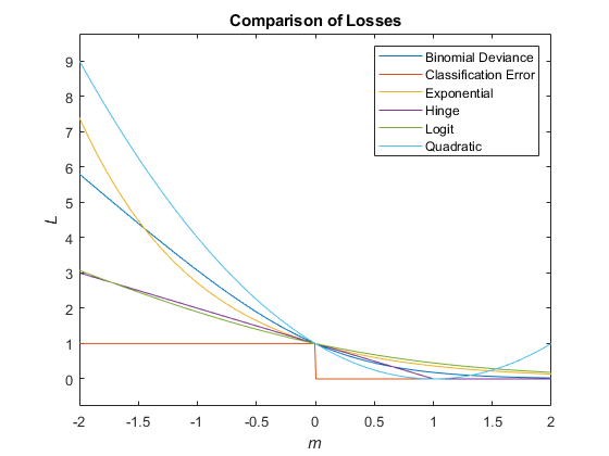
This figure compares the loss functions (except "classifcost", "crossentropy", and "mincost") over the score m for one observation. Some functions are normalized to pass through the point (0,1).

Misclassification Cost

A misclassification cost is the relative severity of a classifier labeling an observation into the wrong class.

Two types of misclassification cost exist: true and expected. Let K be the number of classes.

• True misclassification cost — A K-by-K matrix, where element (i,j) indicates the cost of classifying an observation into class j if its true class is i. The software stores the misclassification cost in the property Mdl.Cost, and uses it in computations. By default, Mdl.Cost(i,j) = 1 if i ≠ j, and Mdl.Cost(i,j) = 0 if i = j. In other words, the cost is 0 for correct classification and 1 for any incorrect classification.

• Expected misclassification cost — A K-dimensional vector, where element k is the weighted average cost of classifying an observation into class k, weighted by the class posterior probabilities.

  $$c_k={\displaystyle \sum _{j=1}^K\widehat{P}}\left(Y=j|x_1,\mathrm{...},x_P\right)Cos{t}_{jk}.$$

  In other words, the software classifies observations into the class with the lowest expected misclassification cost.

Posterior Probability

The posterior probability is the probability that an observation belongs in a particular class, given the data.

For naive Bayes, the posterior probability that a classification is k for a given observation (x₁,...,x_P) is

$$\widehat{P}\left(Y=k|x_1,\mathrm{..},x_P\right)=\frac{P\left(X_1,\mathrm{...},X_P|y=k\right)\pi \left(Y=k\right)}{P\left(X_1,\mathrm{...},X_P\right)},$$

where:

• $$P\left(X_1,\mathrm{...},X_P|y=k\right)$$ is the conditional joint density of the predictors given they are in class k. Mdl.DistributionNames stores the distribution names of the predictors.

• π(Y = k) is the class prior probability distribution. Mdl.Prior stores the prior distribution.

• $$P\left(X_1,\mathrm{..},X_P\right)$$ is the joint density of the predictors. The classes are discrete, so $$P(X_1,\mathrm{...},X_P)={\displaystyle \sum _{k=1}^{K}P}(X_1,\mathrm{...},X_P|y=k)\pi (Y=k).$$

Prior Probability

The prior probability of a class is the assumed relative frequency with which observations from that class occur in a population.

Extended Capabilities

Tall Arrays

Calculate with arrays that have more rows than fit in memory.

This function fully supports tall arrays. You can use models trained on either in-memory or tall data with this function.

For more information, see Tall Arrays.

Version History

Introduced in R2014b