Identify Supercapacitor Parameter
This example shows how to identify the parameters of a supercapacitor. Instead of collecting voltage and current waveforms from a real supercapacitor, this example generates voltage and current waveforms by running a simulation of a supercapacitor using known parameter values. Then the example applies a parameter identification methodology [1] to the waveforms.
To assess the accuracy of the methodology, this example compares the identified parameters to the known parameter values. The example also shows how to further refine the parameter values using the Parameter Estimation app in the Simulink® Design Optimization™ toolbox.
To empirically identify the parameters of an actual supercapacitor, you can:
Collect voltage and current waveforms from the supercapacitor.
Identify parameter values using the waveform data and the methodology in [1].
To identify the parameters of a modeled supercapacitor, this example:
Generates voltage and current waveforms by simulating a model using known values for supercapacitor parameters.
Identifies supercapacitor parameter values using the generated waveform data and the methodology in [1].
Configures and simulates the supercapacitor using the identified supercapacitor parameter values.
To learn how the approach works for a real supercapacitor, evaluate the accuracy of the identification methodology by comparing:
The data you generate using known parameter values and the data you generate using identified parameter values.
The known parameter values and identified parameter values.
If the accuracy is not sufficient, use the Parameter Estimator app from Simulink Design Optimization to improve it. Use the identified parameter values as the starting values for the optimization.
Generate Data
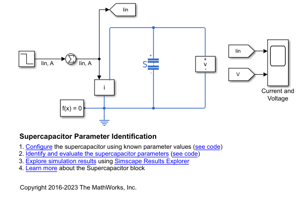
Generate voltage and current waveforms by configuring and simulating a model using known values for the fixed resistances, fixed capacitances, and voltage-dependent capacitor gain parameters of the supercapacitor. Model the input current, configure the physical characteristics and the self-discharge resistance of the supercapacitor using realistic values.
modelName = 'SupercapacitorFromData';
open_system(modelName);
Configure the supercapacitor using known parameter values.
SupercapacitorFromDataParameterConfiguration;
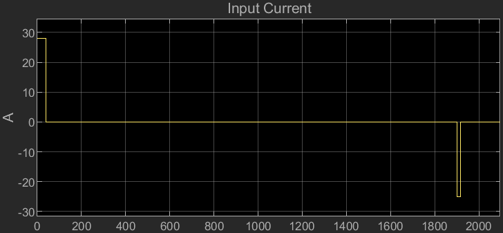
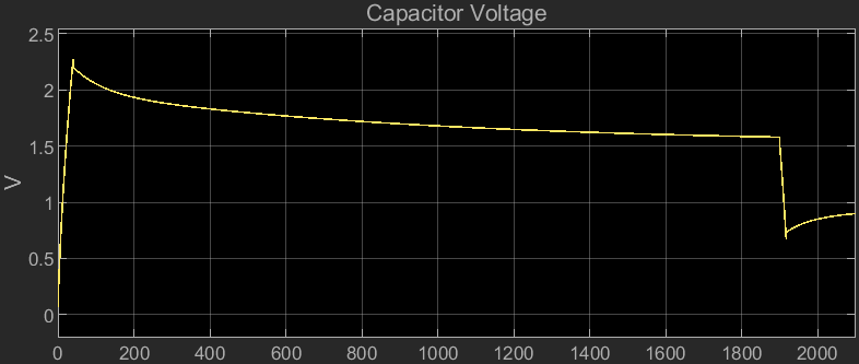
Observe the supercapacitor behavior during three distinct phases:
Charge with constant current
Charge redistribution from immediate to delayed branch
Charge redistribution from immediate and delayed branches to long-term branch
sim(modelName)
Perform Parameter Identification
Using the waveform data from the simulation, apply the methodology described in [1].
Identify Immediate Branch Parameters
During the first stage of the identification, a fully discharged supercapacitor is charged with constant current. The method assumes that the immediate branch stores all the initial charge because the time constant for the branch is relatively small.
To calculate the immediate branch parameters, you take measurements of the charge characteristic. Once the charging current reaches the steady-state at , measure and then calculate the fixed resistance of the immediate branch by using this equation:
where:
is the time at parameter identification event in seconds.
is the terminal voltage at in volts.
is the charging current at in amperes.
is the fixed resistance of immediate branch in ohm.
Once voltage increases from by approximately , measure and and then calculate the fixed capacitance of the immediate branch by using this equation:
where:
is the time at parameter identification event in seconds.
is the terminal voltage at in volts.
is the fixed capacitance of immediate branch in farads.
Once the voltage reaches rated voltage, measure and , and turn off the charging current. After , once charging current reaches steady-state value of measure and and then calculate the voltage-dependent capacitance coefficient by using this equation:
where:
is the time at parameter identification event in seconds.
is the terminal voltage at in volts.
is the time at parameter identification event in seconds.
is the terminal voltage at in volts.
is the voltage-dependent capacitance coefficient in farads per volt.
To perform these calculations, run this script:
SupercapacitorFromDataParameterImmediateIdentification;
Identify Delayed Branch Parameters
During the second stage of the identification, the charge redistributes from the immediate branch to the delayed branch.
To calculate the delayed branch parameters, measure the hold charge characteristics.
Once the voltage decreases from by approximately , measure and and then calculate the delayed branch resistance by using these equations:
where:
is the time at parameter identification event in seconds.
is the terminal voltage at in volts.
is the voltage at which the total immediate capacitance is to be calculated in volts.
is the total immediate capacitance at in farads.
is the delayed branch resistance in ohms.
Wait 300 seconds, measure and and then calculate the delayed branch capacitance by using these equations:
where:
is the time at parameter identification event in seconds.
is the terminal voltage at in volts.
is the total charge supplied to the supercapacitor in coulombs.
is the delayed branch capacitance in farads.
To perform these calculations, run this script:
SupercapacitorFromDataParameterDelayedIdentification;
Identify Long-Term Branch Parameters
During the third and final stage of the identification, the charge redistributes from the immediate and delayed branches to the long-term branch.
To calculate the long-term branch parameters, measure the hold charge characteristics.
Once the voltage decreases from by approximately , measure and and then calculate the long-term branch resistance by using these equations:
where:
is the time at parameter identification event in seconds.
is the terminal voltage at in volts.
is the long-term branch resistance in ohms.
After 30 minutes from the start of the charging/discharging process, measure and and then calculate the long-term branch capacitance by using this equation:
where:
is the time at parameter identification event in seconds.
is the terminal voltage at in volts.
is the long-term branch capacitance in farads.
To perform these calculations, run this script:
SupercapacitorFromDataParameterLongTermIdentification;
Collate Time and Voltage Data
Collate the time and voltage data for each parameter identification event in a MATLAB® table:
DataTable = table((1:8)',...
    [t1 t2 t3 t4 t5 t6 t7 t8]',...
    [v1 v2 v3 v4 v5 v6 v7 v8]',...
    'VariableNames',{'Event','Time','Voltage'})
DataTable=8×3 table
    Event     Time      Voltage
    _____    _______    ________

      1         0.02    0.071799
      2      0.51803      0.1218
      3           40      2.2717
      4        40.02      2.2019
      5       56.675      2.1519
      6       356.67      1.8473
      7       499.28      1.7973
      8         1800      1.5865
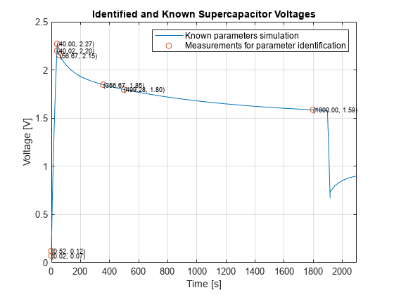
SupercapacitorFromDataPlotVoltage;
![Figure contains an axes object. The axes object with title Identified and Known Supercapacitor Voltages, xlabel Time [s], ylabel Voltage [V] contains 10 objects of type line, text. One or more of the lines displays its values using only markers These objects represent Known parameters simulation, Measurements for parameter identification.](../../examples/simscapeelectrical/win64/SupercapacitorFromDataExample_05.png)
Evaluate Accuracy of Identified Parameters
Configure and simulate the model using the identified supercapacitor parameters. Then, to evaluate the accuracy of the identified parameter values, compare the waveform output to the data that you generate by running a simulation that uses known parameters.
SupercapacitorFromDataParameterSimulateIdentifiedParameters;
![Figure contains an axes object. The axes object with title Identified and Known Supercapacitor Voltages, xlabel Time [s], ylabel Voltage [V] contains 3 objects of type line. One or more of the lines displays its values using only markers These objects represent Known parameters simulation, Measurements for parameter identification, Identified parameters simulation.](../../examples/simscapeelectrical/win64/SupercapacitorFromDataExample_07.png)
Optimize Parameters Using Parameter Estimation App
To perform the optimization of the supercapacitor parameters, you must have the Simulink Design Optimization toolbox installed.
If the traces are not similar enough to meet requirements, then the identified parameter values can serve as initial parameter values for the Parameter Estimator app from Simulink Design Optimization.
To optimize the super capacitor parameters, at the MATLAB Command Window, enter:
spetool('SupercapacitorSDOParameterEstimatorSession');
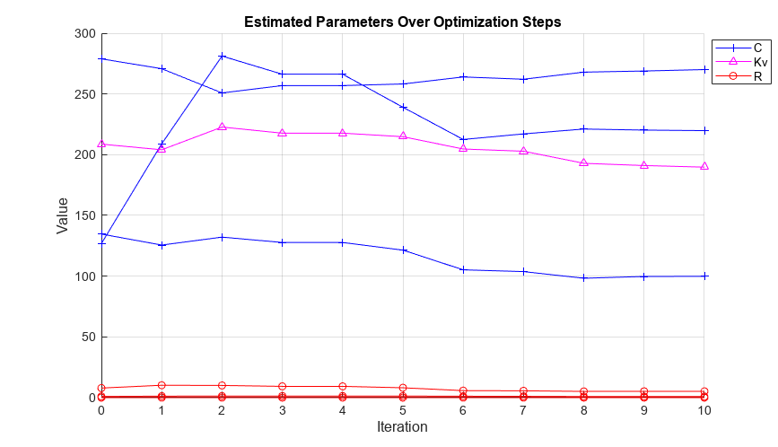
Display Optimization Results
Display the parameter trajectory created using the Sum Squared Error cost function and Nonlinear least squares optimization method.
openfig('SupercapacitorSDOParameterEstimatorResults');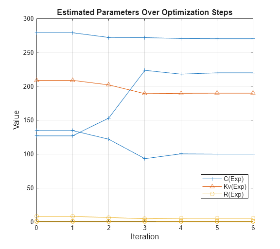
References
[1] Zubieta, L. and R. Bonert. "Characterization of Double-Layer Capacitors for Power Electronics Applications." IEEE Transactions on Industry Applications, Vol. 36, No. 1, 2000, pp. 199-205.