Create and Run Real-Time Application from Simulink Model

R2026b

This example shows how to visualize signals by various means in non-real-time (NRT) and real-time (RT) models. Most importantly, this example demonstrates how to instrument signals (add signals to an instrument) for visualization without marking signals for logging or connecting signals to File Log blocks.

To complete the steps in this example, you must already know how to create, configure, and simulate such a model. As you go through the example, you transform slrt_ex_osc_nrt into a Simulink Real-Time™ model configured to build as a real-time application. You then build, download, and execute the real-time application on your target computer.

Open the Non-Real-Time Model

Open the NRT Simulink® model of a damped oscillator, slrt_ex_osc_nrt. In the MATLAB® Command Window, type:

model_nrt = 'slrt_ex_osc_nrt';
open_system(model_nrt);

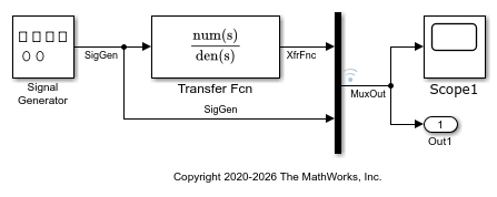
This NRT model, which is configured for the Simulink® Coder™ grt.tlc system target file (STF), lets you visualize signals by using the Scope block or by using the MuxOut signal that is marked for streaming to the Simulation Data Inspector.

Open the RT Simulink® Real-Time model of a damped oscillator, slrt_ex_osc_rt. In the MATLAB Command Window, type:

model_rt = 'slrt_ex_osc_rt';
open_system(model_rt);

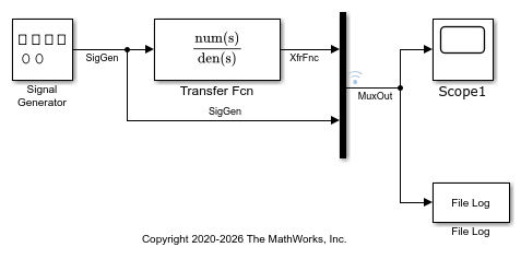
This RT model, which is configured for a Simulink Real-Time (STF) such as speedgoat.tlc, lets you visualize signals by using the Scope block, by using the MuxOut signal that is marked for streaming to the Simulation Data Inspector, or by using Simulink Real-Time instrumented signals that you add to the real-time application.

Start Target Computer and Display Status Monitor

Boot the RTOS on the target computer and display the status monitor.

Starting the target computer boots the RTOS. The target computer waits for the Simulink Real-Time software to download and start a real-time application from the development computer or to start a real-time application that was previously downloaded.

After you have configured the Simulink Real-Time product by using the Simulink Real-Time Explorer, you can start the target computer and connect the development computer to the target computer. Before building the real-time application, you start the target computer. After the build process is complete, you download the real-time application to the target computer.

The status monitor application on the target computer displays status of the real-time application and other target computer status information. The target computer display supports multiple sessions. You can choose to display the status monitor (default, session 1) or display the target computer command line interface (session 2). To display the target computer status monitor:

Start the target computer.
The target computer displays session 1 (default) and the target computer status monitor.
Connect to the target computer. In the MATLAB Command Window, type:

tg = slrealtime;
connect(tg);

To view the status monitor from the development computer, you can use PuTTY to open an SSH client and start the status monitor application /usr/target/bin/statusmonitor on the target computer.

For more information, see Target Computer Status Monitor.

Transform Simulink Model to Simulink Real-Time Application

Set configuration parameters for building a Simulink model as a real-time application.

To run a Simulink model as a real-time application under Simulink Real-Time, configure the system target file in the configuration parameters to match the target computer and configure parameters for code generation and target execution.

The example model, slrt_ex_osc_ucf, is a non-real-time model of a damped oscillator. You enter the simulation and real-time run parameters in the Configuration Parameters dialog box. These parameters provide information to Simulink Coder™ on how to build a real-time application from the Simulink model.

After you open a Simulink model and start the target computer, you can enter the simulation parameters.

In the MATLAB Command Window, type slrt_ex_osc_ucf.
In Simulink Editor, from the Apps tab, click Simulink Real-Time.
From the Real-Time tab, click Hardware Settings.
In the Configuration Parameters dialog box, click the Solver node.
In the Solver selection section, from the Type list, select Fixed-step.
From the Solver list, select a solver. For example, select the general-purpose solver ode4 (Runge-Kutta).
Under Solver details, in the Fixed-step size (fundamental sample time) box, enter the sample time for the real-time application. For example, enter 0.00025 seconds (250 microseconds). After creating the real-time application, you can change this value. If you find that a value overloads the CPU on the target computer, try a larger Fixed-step size value, such as 0.0002 seconds. The sample times of the model blocks can be multiples only of Fixed-step size. If you enter 'auto' in Fixed-step size, the fundamental sample time is calculated from the sample times of the model blocks.
Click OK.
From the Apps tab, select Simulink Real-Time. This selection configures the system target file (STF) and other model settings for Simulink Real-Time. If applying this setting in the MATLAB Command Window, use the configureModelForTarget Platform function.
In the Simulation tab, from the Save button, click Save As.
Enter a file name. For example, enter slrt_ex_osc_rt.

Build Real-Time Application from Model

In the slrt_ex_osc_rt model, unmark signals that have been marked for data logging. Then, remove the File Log block and the unused signal path. Configure the model for target computer tg and build the real-time application MLDATX file from the model.

model = 'slrt_ex_osc_rt';
modelSTF = getSTFName(tg);
set_param(model,"SystemTargetFile",modelSTF);
evalc('slbuild(model)');

Add Signals to Instruments for Data Visualization

Add signals SigGen and XfrFnc to instrument tgInst in Target object tg. The data from these signals is added to file logging for the real-time application.

mldatxname = 'slrt_ex_osc_rt.mldatx';
tgInst = slrealtime.Instrument(mldatxname);
tgInst.Name = 'TargetInstrument';
addSignal(tgInst,'SigGen');
addSignal(tgInst,'XfrFnc');
addForFileLog(tg.Instruments,tgInst);

An advantage of using instruments for streaming or logging signals is that you do not need to mark signals for streaming or add File Log blocks for logging. With instrumented signals, you can programmatically control the selection of signals for visualization.

Run Real-Time Application and View Signal Data

Load and start the real-time application. When the application status changes to stopped, auto import the file log data and view the signal data in the Simulation Data Inspector.

load(tg,model);
start(tg,'AutoImportFileLog',true);
while ~strcmp(tg.status,'stopped')
    pause(5);
end
stop(tg);
Simulink.sdi.view

  Importing Log file 1 of 1 ...

Remove Instrument and Close Models

removeForFileLog(tg.Instruments,tgInst);
bdclose(model_nrt);
bdclose(model_rt);