Import Command-Line Objects into Sensitivity Analyzer Programmatically

This example shows how to create objects through the command-line functionality and import them into the Sensitivity Analyzer app using sdo.SessionInterface.

You can set up a sensitivity analysis problem in the Sensitivity Analyzer app by following the UI workflow. Sometimes, when you want to specify a large number of parameters along with their probability distributions or specify a large number of requirements, this process becomes tedious. You can specify the parameters and requirements using the command-line functionality instead. Then, you can import the parameters and requirements into the Sensitivity Analyzer app using sdo.SessionInterface.

Initiate Problem Specification in the App

Open the Simulink® model.

open_system('spe_muscle')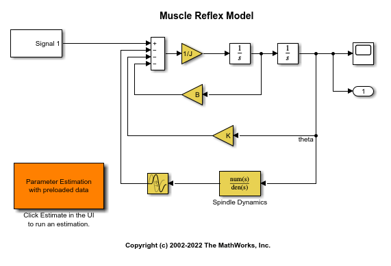

To open a blank Sensitivity Analyzer app session for the model, in the Apps tab, click Sensitivity Analyzer, or enter this command at the MATLAB® command line.

ssatool('spe_muscle')

Define one requirement and a parameter set with one parameter.

• To define a parameter set, in the Sensitivity Analysis tab, in the Select Parameters menu, click New. In the Select Parameters dialog box, select the parameter B and click OK. To select a probability distribution for B and generate values for the parameter, in the Sensitivity Analysis tab, in the Generate Values menu, click Generate Random Values. In the Generate Random Parameter Values dialog box, specify the Number of Samples as 100 and the Distribution as Normal. Specify the mean, mu, to be 3 and the standard deviation, sigma, to be 0.2. Click OK to generate the values.

• To define a requirement, in the Sensitivity Analysis tab, in the New Requirement menu, click Signal Bound. In the Create Requirement dialog box, in the Specify Signal Bound section, specify the Start Time as 0, the End Time as 5, and the Start Amplitude and End Amplitude as 0.05. In the Select Signals to Bound section, specify the signal to which the bound applies. Click the Add button () and select the theta signal in the model. In the Create Signal Set dialog box, click OK.

When there are many additional parameters, distributions, and requirements, specifying all of them directly in the app can be tedious. Instead, you can define them in the command line and import them into the app.

Define Parameters in Command Line

Create a blank session sdo.SessionInterface object to interface with both the app and the objects defined in the command line.

si = sdo.SessionInterface('spe_muscle','SensitivityAnalysis');

Define all the model parameters to be estimated in the command line as a vector of param.Continuous objects. Because one of the parameters, tau, is a time constant, specify that it cannot be negative.

params = [...
    param.Continuous('B',3) ; ...
    param.Continuous('alpha',0.2) ; ...
    param.Continuous('beta',0.1) ; ...
    param.Continuous('tau',0.005)];
params(4).Minimum = 0;

Create an object to store the parameters and their probability distributions using sdo.ParameterSpace. Specify a quasi-random approach for the sampling. This approach samples the space efficiently and has the potential to use a smaller sample size while obtaining valid analysis results.

ps = sdo.ParameterSpace(params);
ps.ParameterDistributions(1) = makedist('Normal','mu',3,'sigma',0.2);
ps.ParameterDistributions(4) = makedist('Exponential','mu',2);
ps.Options.Method = 'sobol';

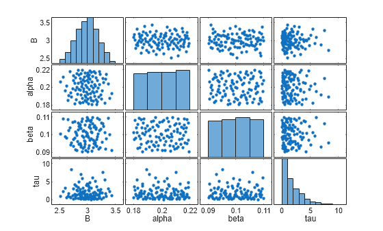
Use the parameter space to generate sample values. To visualize the sample space, make a scatter plot using sdo.scatterPlot.

sampleOutput = sample(ps,100);
sdo.scatterPlot(sampleOutput.X);

Create a structure to store the parameters, parameter space, and values. Assign this structure to the Parameters property of the session interface object.

paramset = struct( ...
    'Parameters', params, ...
    'ParameterSpace', ps, ...
    'Values', sampleOutput.X);
si.ParameterSet = paramset;

Define Requirements in Command Line

Define requirement specifications in the command line using sdo.requirements.SignalBound.

ReqSpecifications = sdo.requirements.SignalBound( ...
    'BoundTimes', [0 5], 'BoundMagnitudes', [0.05 0.05]);
ReqSpecifications(2) = sdo.requirements.SignalBound( ...
    'BoundTimes', [0 1], 'BoundMagnitudes', 0.01*[1 1]);
ReqSpecifications(3) = sdo.requirements.SignalBound( ...
    'BoundTimes', [2 3], 'BoundMagnitudes', -0.03*[1 1], 'Type','>=');
ReqSpecifications(4) = sdo.requirements.SignalBound( ...
    'BoundTimes', [2.7 3.5], 'BoundMagnitudes', 0.017*[1 1]);

Specify the model signal to which the requirements apply using Simulink.SimulationData.Signal.

Sig = Simulink.SimulationData.Signal;
Sig.BlockPath = 'spe_muscle/Integrator';
Sig.PortType = 'outport';
Sig.PortIndex = 1;
Sig.Name = 'theta';

Create a structure to store the requirement specifications. In this example, all requirements apply to the same signal. Specify this signal as the source for each requirement. Assign the created structure to the Requirements property of the session interface object.

reqs = struct;
for ct = 1:numel(ReqSpecifications)
    reqs(ct).Name = ['Req' num2str(ct)];
    reqs(ct).Specification = ReqSpecifications(ct);
    reqs(ct).Source = {Sig};
end
si.Requirements = reqs;

Plot Requirements

Before importing the objects defined in the command line into the app, plot the requirements to make sure they look correct. Along with the requirement bounds, plot the model output. To do this, log the model output so that after simulation you can retrieve the log to plot the signal.

ModelOutput = Simulink.SimulationData.SignalLoggingInfo;
ModelOutput.BlockPath = 'spe_muscle/Integrator';
ModelOutput.OutputPortIndex = 1;
ModelOutput.LoggingInfo.NameMode = 1;
ModelOutput.LoggingInfo.LoggingName = 'ModelOutput';

To store the logging information and simulate the model, create an sdo.SimulationTest object.

Simulator = sdo.SimulationTest('spe_muscle');
Simulator.LoggingInfo.Signals = ModelOutput;
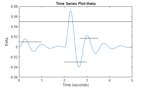
Simulator = sim(Simulator);

Plot the model signal and the requirement bounds that the signal should ultimately satisfy.

SimLog = find(Simulator.LoggedData, ...
    get_param('spe_muscle','SignalLoggingName'));
SignalLog = find(SimLog,'ModelOutput');
plot(SignalLog.Values.Time,SignalLog.Values.Data);
for ct = 1:numel(ReqSpecifications)
    line(ReqSpecifications(ct).BoundTimes, ReqSpecifications(ct).BoundMagnitudes,'Color','black');
end
xlabel('Time (seconds)')
ylabel('theta')
title('Time Series Plot:theta')

Import Command-Line Objects into the App

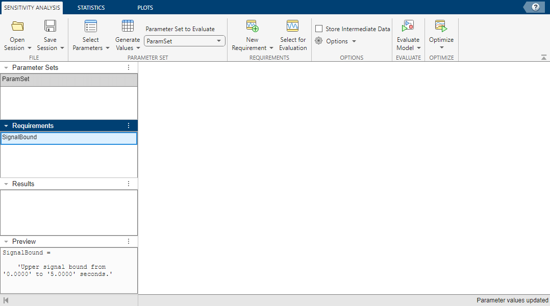
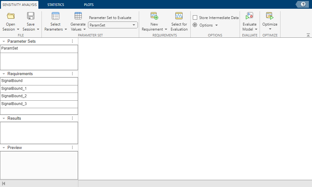
Import the objects defined in the command line into the app using sdotool. This action launches the app.

sdotool(si);

You can see that the app is populated with the parameter set and all the requirements.

Close the model.

bdclose('spe_muscle')