Create LPV Pendulum Model Using Batch Linearization

Since R2025a

This example shows how to create a linear parameter-varying (LPV) model from a Simulink® pendulum model. In this example, you:

1. Batch linearize the nonlinear pendulum model at several operating points.

2. Construct an LPV model from the batch linearization result.

3. Compare the response of nonlinear, LPV, and small angle linear approximation models.

Load the model.

mdl = "scdPendulumNoWrap";
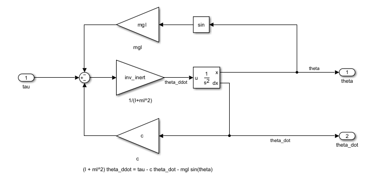
load_system(mdl);

For this physical pendulum model, the dynamics are defined by:

$\left(\mathit{I}+{\mathit{ml}}^2\right)\ddot{\theta }=\tau -\mathit{c}\dot{\theta }-\mathit{mgl}\times \sin \left(\theta \right)$.

Here,

• $\mathit{I}$ is the moment of inertia about the pivot.

• $\mathit{l}$ is the distance from the pivot point to the center of mass of the pendulum.

• $\mathit{m}$ is the mass of the pendulum.

• $\theta$ is the angular displacement of the pendulum from the vertical and is measured starting from the stable equilibrium, where the mass is hanging straight down.

• $\tau$ is the external torque applied to the pendulum.

• $\mathit{c}$ is the damping coefficient.

• $\mathit{g}$ is the acceleration due to gravity.

Specify model parameters.

tau0 = 0;
mgl = 1;
inv_inert = 1;
c = 0.1;
theta0 = pi/8;
dtheta0 = 0;

Specify the input torque as linearization input and the angle $\theta$ as output.

io(1) = linio(mdl+"/tau",1,"input");
io(2) = linio(mdl+"/pendulum",1,"output");

Create the operating point grid theta = [$-\pi$,$\pi$] with 21 equally spaced points.

theta_grid = linspace(-1,1,21)'*pi;
N = numel(theta_grid);
clear op
for i = N:-1:1
    if i == N
        op_ = operpoint(mdl);
    else
        op_ = copy(op(end));
    end
    op_.States(1).x = theta_grid(i);
    op(i,1) = op_;
end

Consistent and uniform state dimensions, delay modeling, and offset handling across the linearization grid are required when building LPV models. To perform state-consistent reduction, enable the BatchConsistency option. Additionally, store the linearization offsets in the Offsets property of the state-space model array.

options = linearizeOptions(BatchConsistency=true,StoreOffsets="system");

Linearize the model.

sys = linearize(mdl,io,op,options);
size(sys)

21x1 array of state-space models.
Each model has 1 outputs, 1 inputs, and 2 states.

To specify the parameter dependence of the models in sys, use the SamplingGrid property of the state-space object. Here, the dependence is on $\theta$.

sys.SamplingGrid = struct(theta=theta_grid);

To create the interpolated LPV model, use ssInterpolant.

lpv_sys = ssInterpolant(sys);

You can now simulate the LPV model response. Specify a time vector up to 25 seconds and zero torque input for simulation.

t = 0:0.1:25;
u = 0.*t;

To simulate the LPV model using lsim, you must also specify an initial condition for the states and a parameter trajectory $\mathit{p}\left(\mathit{t}\right)$ implicitly as a function $\mathit{F}\left(\mathit{t},\mathit{x},\mathit{u}\right)$ of time $\mathit{t}$, input $\mathit{u}$, and state $\mathit{x}$. Here $\mathit{p}\left(\mathit{t}\right)$ is just the first state $\theta \left(\mathit{t}\right)$.

IC = [theta0;dtheta0];
p = @(t,x,u) x(1);
y = lsim(lpv_sys,u,t,IC,p);

To compare the models, you can use the preconfigured model ComparePendulumModels.slx provided with this example.

load_system("ComparePendulumModels");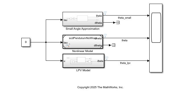

This model contains three subsystems.

• Linear model created using small angle approximation of the original model with $\sin \left(\theta \right)\simeq \theta$.

• Original nonlinear model.

• LPV model implemented using an LPV System block. The block takes the batch linearization result sys and simulates the LPV models in Simulink®.

Simulate the model and store the simulation data.

in = Simulink.SimulationInput("ComparePendulumModels");
out = sim(in);

Plot the responses from the simulation data.

figure(1)
th = getElement(out.logsout,'theta');
plot(th.Values);
hold on
th_LPV = getElement(out.logsout,'theta_lpv');
plot(th_LPV.Values);
plot(t,y);
th_sm = getElement(out.logsout,'theta_small');
plot(th_sm.Values,"--");
legend(["Nonlinear","LPV (block)","LPV (ssInterpolant)","Small angle approximation"]);
title("Model Comparison")

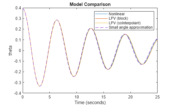
Here, the LPV models provide a good approximation of the nonlinear model. The small angle approximation is also good, however, this is only the case because the initial condition ${\theta }_0$ is a small angle pi/8. The small angle approximation gets worse as you increase ${\theta }_0$. For example, set theta0 to pi/2, and run this example again. You get the result shown in the following figure.

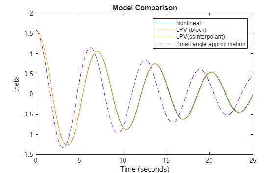
As you can see, the deviation from the nonlinear model gets much larger as the simulation progresses. Whereas, the LPV model continues to provide an accurate approximation of the nonlinear model.