Linearize Sparse Models
You can obtain a sparse linear model from a Simulink® model that contains a Sparse Second Order or Descriptor State-Space block. Linearizing such models produces one of the following sparse state-space objects.
mechssmodel when you use a Sparse Second Order blocksparssmodel when you use a Descriptor State-Space block and configure the block to linearize to a sparse model
For more information on sparse models, see Sparse Model Basics.
For a command-line linearization example, see Linearize Simulink Model to a Sparse Second-Order Model Object.
The Sparse Second Order block always linearizes to a
mechss model. As a result, the overall linearized model is a
second-order sparse model when this block is present.
To linearize a Descriptor State-Space block to a sparse model, select the Linearize to sparse model block parameter.
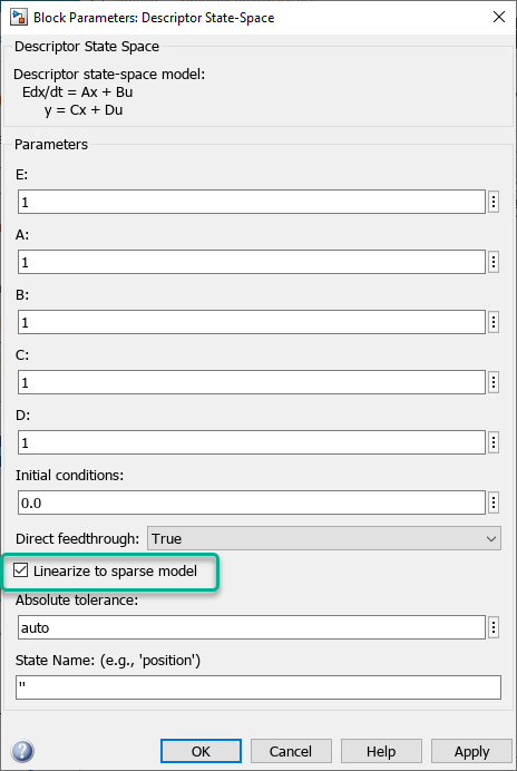
You can also select this parameter programmatically. Here, blockpath is
the path to the Descriptor State-Space block.
set_param(blockpath,'LinearizeToSparse','on')
The Linearize to sparse model parameter of the Descriptor State-Space block is ignored when you specify a custom linearization for the block.
Linearize Sparse Models at the Command Line
You can linearize a model that contains a sparse block at the command line using either
the linearize function or an slLinearizer interface.
To analyze the resulting linearized model in the:
Time domain, you must specify a time vector or a final simulation time. For example, plot the step response of linearized sparse model
linsysfor 10 seconds using 100 sample points.t = linspace(0,10,1000); step(sys,t)
Frequency domain, you must specify a frequency vector. For example, plot the Bode response of linearized sparse model
linsysfrom 101 to 105 rad/sec using 1000 logarithmically spaced frequency points.w = logspace(1,5,1000); bode(linsys,w)
For more information on analyzing sparse models at the command line, see Sparse Model Basics.
Linearize Sparse Models Using Model Linearizer
You can interactively linearize a model that contains a sparse block using the Model Linearizer app.
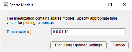
Each time you plot a time-domain or frequency-domain response of the resulting linearized model, Model Linearizer prompts you to enter a time or frequency vector for plotting. For example:
Time domain — Plot response for 10 seconds in 0.01 second increments.
Frequency domain — Plot response from 10–1 to 103 rad/sec using 100 logarithmically spaced frequency points.
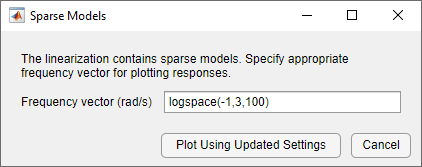
You cannot change the time or frequency vector for an existing sparse model response plot. Instead, create a new plot for the same sparse model using an updated time or frequency vector.
To view the structure of the linearized sparse model, export the model to the
MATLAB® workspace and use the spy and
showStateInfo
functions.
Limitations
Sparse linearization has the following limitations.
If you disable block reduction when linearizing a sparse model, the resulting linear model is a dense
ssmodel object.Due to simulation limitations, snapshot linearization might not work when your model contains a Descriptor State-Space or Sparse Second Order block.
Sparse linearization is incompatible with block substitutions involving tunable or uncertain models, such as
genssoruss(Robust Control Toolbox), respectively.When analyzing linearized sparse systems, Pole-Zero Map and I/O Pole-Zero Map plots are not supported.
See Also
Blocks
Functions
sparss|mechss|linearize|slLinearizer