Compute Operating Points from Specifications Using Model Linearizer
You can compute a steady-state operating point of a Simulink® model by specifying constraints on the model states, outputs, and inputs, and finding a model operating condition that satisfies these constraints. For more information on steady-state operating points, see About Operating Points and Compute Steady-State Operating Points.
To find an operating point for your Simulink model, you can interactively trim your model using Model Linearizer, as shown in this example.
Alternatively, you can trim your model:
In Steady State Manager. For more information, see Compute Operating Points from Specifications Using Steady State Manager.
At the command line. For more information, see Compute Operating Points from Specifications at the Command Line.
In this example, you compute an operating point to meet state specifications. Using a similar approach, you can define output or input specifications. Also, you can define a combination of state, output, and input specifications; that is, you do not have to use, for example, only state specifications.
For more information on trimming your model to meet specifications, see Compute Steady-State Operating Points from Specifications.
Open Model Linearizer
Open the Simulink model.
openExample("scdspeed")
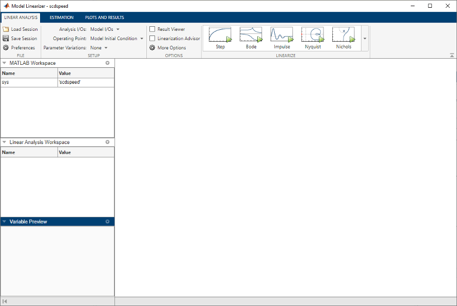
To open the Model Linearizer, in the Simulink model window, in the Apps gallery, click Model Linearizer.
Define Operating Point Specifications
In Model Linearizer, on the Linear Analysis
tab, in the Operating Point drop-down list, select
Trim Model.
In the Trim the model dialog box, on the Specifications tab, you can define specifications for model states, inputs, and outputs. For this example, click the States tab.
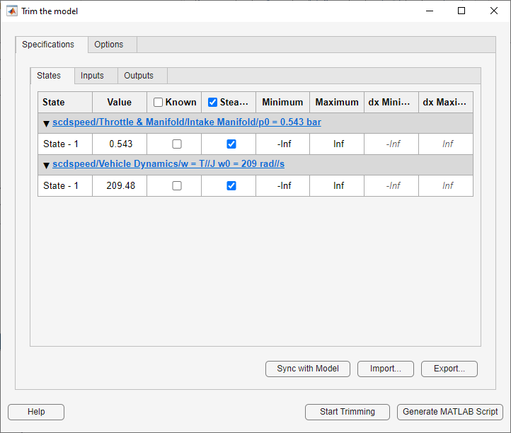
By default, on the States tab, the app specifies both model states to be at equilibrium, as shown by the check marks in the Steady State column. Both states are also specified as unknown values; that is, their steady-state values are calculated during trimming, with an initial guess specified in the Value column.
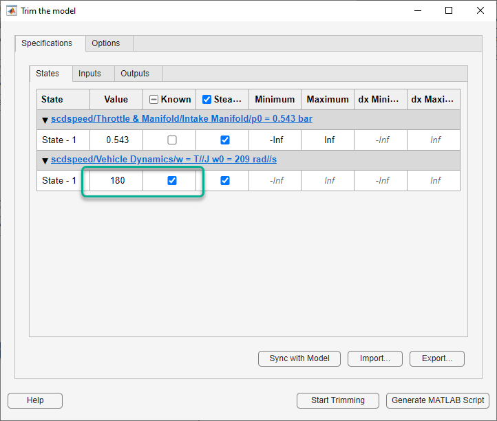
Change the second state, the engine angular velocity, to be a known value.
In the Known column, select the corresponding row and,
in the Value column, set the value to
180.
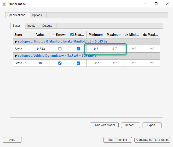
You can also specify bounds for model states during trimming. For this
example, constrain the first state to be between 0.5 and
0.7. To do so, enter these values in the
Minimum and Maximum columns,
respectively.
Trim Model
To compute an operating point that meets these specifications, click Start trimming.
The software uses an optimization search to find the operating point that meets your specifications.
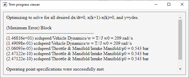
The Trim progress viewer shows the optimization progress and that the optimization algorithm terminated successfully. The (Maximum Error) column shows the maximum constraint violation at each iteration. The Block column shows the block to which the constraint violation applies.
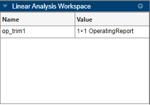
The trimmed operating point, op_trim1, appears in the
Linear Analysis Workspace.
To evaluate whether the resulting operating point values meet the
specifications, in the Linear Analysis Workspace,
double-click op_trim1.
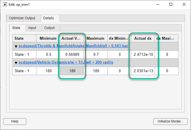
In the Edit dialog box, on the State tab, the
Actual Value for the first state falls within the
Desired Value bounds, and the actual angular
velocity is 180, as specified.
The Actual dx column shows the rates of change of the state values at the operating point. Since these values are near zero the states are not changing, showing that the operating point is in a steady state.
Constrain State Derivatives
When you trim your model to meet state specifications, you can also constrain the derivatives of states that are not at steady state. Using such constraints, you can trim derivatives to known nonzero values or specify derivative tolerances for states that cannot reach steady state.
For example, suppose you want to find the operating condition at which the
engine angular velocity is 180 rad/s and the angular acceleration is
50 rad/s2. To do so,
first open the Trim the model dialog box. In the Model
Linearizer, in the Operating Point drop-down
list, select Trim Model.
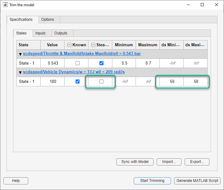
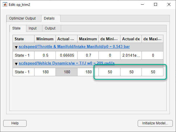
In the Steady State column, clear the selection in the
corresponding row. Then, in the dx Minimum and
dx Maximum columns, set both state derivative
bounds to 50.
To compute the operating point, click Start trimming.
In the Linear Analysis Workspace, double-click
op_trim2.
In the Edit dialog box, in the second row, the Actual dx column matches the Desired dx column. Therefore, the operating point meets the specified state derivative constraints.
After trimming your model, you can:
Linearize your model at the resulting operating point. For more information, see Linearize at Trimmed Operating Point.
Simulate your model at the resulting operating point. For more information, see Simulate Simulink Model at Specific Operating Point.