Arithmetic Operations on Matrix Signals

This example shows how to perform arithmetic operations on signals carrying matrix and vector data.

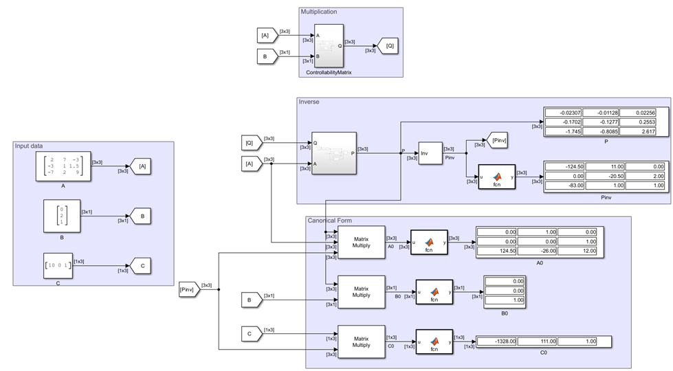
In this example, the model performs a series of matrix operations on the input matrices and vectors to transform a system with state-space representation to its controllable canonical form, also known as phase variable form. The phase variable form provides a simplified representation of the system that eases the controllability analysis and helps in model reduction.

The sstocanonical model contains these components that show different mathematical operations.

• Input data

• Multiplication

• Inverse

• Canonical Form

Open the model.

mdl = "sstocanonical.slx";
open_system(mdl)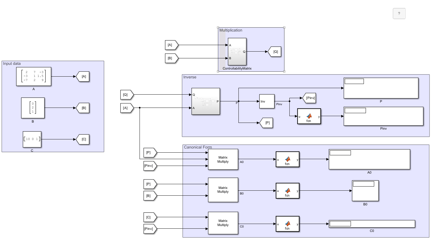

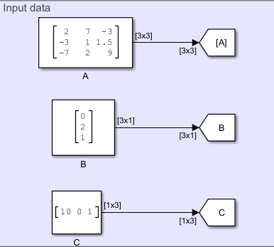
Input Data

The Input data component represents the input matrix and vectors in state-space form.

$$\underset{}{\overset{\dot{}}{x}}=Ax+Bu$$

$$y=Cx+Du$$

In this example, $$A$$ is 3-by-3 matrix that represents the system, $$B$$ is 3-by-1 input vector, $$C$$ is 3-by-1 output vector, and the model assumes $$D$$ to be 0.

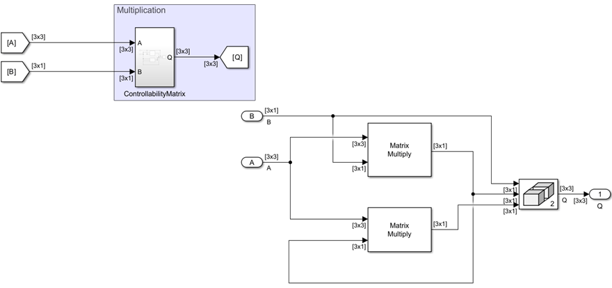
Multiplication

The controllability matrix for the state-space system is defined as:

$$Q=[BAB{A}^{2}B.....A^{n-1}B]$$, where n represents the number of states.

The Multiplication component computes the controllability matrix Q from the state-space system.

Controllable Canonical Form

The model modifies the state-space equation using the substitution $$x=P^{-1}z$$ and $$D=0$$ as:

$$\underset{}{\overset{\dot{}}{z}}=PA{P}^{-1}z+PBu$$

$$y=C{P}^{-1}z$$

In these equations, $$P=[P_1{P}_{1}A{P}_1{A}^2]$$, where $$P_1$$ is the last row of $$Q_{inv}$$. The Inverse component computes the inverse of the controllability matrix Q and transformation matrix P.

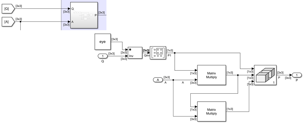
The equation is further simplified as:

$$\underset{}{\overset{\dot{}}{z}}=A_0+B_{0}u$$

$$y=C_{0}z$$

where $$A_0=PA{P}^{-1}$$, $$B_0=PB$$, and $$C_0=C{P}^{-1}$$.

The Canonical Form component computes the canonical form of the state-space system.

Simulation and Results

Simulate the model and visualize $$A_0$$, $$B_0$$, $$C_0$$ using Display blocks.

out = sim(mdl);

Verification Using MATLAB

You can verify the simulation result by comparing it with the controllable canonical form of the system obtained programmatically using MATLAB functions. Observe that, first the ss2tf function is used to obtain the transfer function coefficients.

A = [ 2 7 -3
    -3 1 1.5
    -7 2 9];
B = [0
    2 
    1];
C = [10 0 1];

D = 0;

[b,a] = ss2tf (A,B,C,D);

Then, the transfer function coefficients are used from the arrays b and a to obtain the controllable canonical form of the system. Observe that the matrices match the simulation results.

$${\alpha }_2=-12.00,{\alpha }_1=26.00,{\alpha }_0=-124.50$$

$${\beta }_2=1.00,{\beta }_1=111.00,{\beta }_0=-1328.00$$

$$A_0=\left(\begin{array}{ccc}0& 1& 0\\ 0& 0& 1\\ 124.50& -26.00& 12.00\end{array}\right)$$

$$B_0=\left(\begin{array}{c}0\\ 0\\ 1\end{array}\right)$$

$$C_0=\left(\begin{array}{c}-1328.00111.001.00\end{array}\right)$$

References

[1] Ramaswami, B., and K. Ramar. "Transformation to the phase-variable canonical form." IEEE Transactions on Automatic Control 13, no. 6 (1968): 746-747. https://doi.org/10.1109/TAC.1968.1099061.