Analyze Impact of Model Parameters on Bouncing Ball Simulation
This example analyzes the impact of the damping coefficient on a mass-spring-damper model of the dynamics of a bouncing ball. The example runs a set of simulations. Each simulation uses a different value of the parameter that represents the damping coefficient. By visualizing and postprocessing the results of the simulations, the example explores these questions:
How does the damping affect the position of the ball throughout the simulation?
How do the states of the system change throughout the simulation?
Does the damping affect the number of times the ball bounces?
Does the damping affect the timing of the bounces?
The effect a parameter has in a simulation depends on how the parameter relates to the system equations that govern the behavior of the model. Some parameters can have a significant effect on simulation results, performance, or stability. By running parameter sweep simulations, you can:
Simulate and analyze multiple designs.
Tune and optimize parameter values.
Simulate and analyze the model under different conditions.
Mass-Spring-Damper Model of Bouncing Ball
To model the dynamics of a bouncing ball, consider the forces that act on the ball.
When the ball is in the air, only the force due to gravity acts on the ball.
When the ball is in contact with the surface, both the force due to gravity and the force from the collision with the surface act on the ball.
The difference in the system dynamics based on the position of the ball makes the bouncing ball an example of a hybrid dynamic system. Hybrid dynamic systems have both continuous dynamics and discrete transitions at which the system dynamics change and the system state values can "jump" or have discontinuities. In the model of the bouncing ball, the discrete transitions occur when the ball makes contact with the surface on which it bounces and when the ball bounces off of the surface into the air.
These equations represent the dynamics of the bouncing ball when the ball is in the air:
where is the acceleration due to gravity, is the velocity of the ball, and is the position of the ball.
The example Simulation of Bouncing Ball models the interaction of the ball with the surface on which it bounces using a single parameter, the coefficient of restitution. The coefficient of restitution represents the energy loss and restoring force of each bounce. This example models the collision of the ball with the surface as a mass-spring-damper system with nonlinearity.
The mass-spring-damper approach represents the interaction of the ball and surface with higher fidelity, incorporating compression and deformation that occurs during the collision. With this approach, the position of the ball can become negative as a result of the ball compressing and the surface bending or compressing on impact.
This second-order differential equation represents the dynamics of the bouncing ball when the ball is in contact with the surface using a mass-spring-damper approach:
where:
is the first derivative of the position, which corresponds to the velocity of the ball
is the second derivative of the position, which corresponds to the acceleration of the ball
is the acceleration due to gravity
is the mass of the ball
represents the linear stiffness of the ball and the surface on which it bounces
represents damping in the interaction between the ball and the surface
represents nonlinearity in the restoring force
You can also represent the system using two first-order equations:
When , the equation becomes linear, leaving only the linear damping and stiffness coefficients and . This example analyzes the impact of the damping coefficient .
Open Simulink Model
Open the model ModelParameterImpact, which implements the mass-spring-damper model of the bouncing ball.
mdl = "ModelParameterImpact";
open_system(mdl)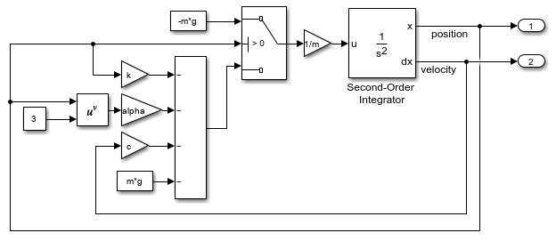
A Switch block models the discrete transition in the bouncing ball dynamics based on the position of the ball.
When the position of the ball is greater than 0, only gravity contributes to the acceleration of the ball.
When the position of the ball is less than or equal to zero, gravity, the mass-spring-damper terms, and the nonlinear term contribute to the acceleration of the ball.
The Second-Order Integrator block computes the position and velocity of the ball, and two Outport blocks create output ports for the position and velocity signals. Constant blocks, Gain blocks, and mathematical function blocks implement the other terms in the system equations.
To parameterize the model, the Value parameters of the Constant blocks, the Gain parameters of the Gain blocks, and the initial state parameters of the Second-Order Integrator block are defined using variables. Because the Output model configuration parameter is enabled by default, the Outport blocks log the position and velocity signals during simulation.
Simulate Several Parameter Values
This example runs a set of simulations that each use a different value of the damping coefficient . First, define the values of the model parameters in the workspace. Then, create an array of Simulink.SimulationInput objects to specify the value of the damping coefficient to use in each simulation.
The table summarizes the parameter values used in this example. The damping coefficient is a vector that contains the value used in each simulation.
Variable Name | Parameter Value | Units | Description |
|---|---|---|---|
| 9.81 | Acceleration due to gravity | |
| 2000 | Stiffness of the surface and ball | |
| 2 | Nonlinearity in restoring force | |
| 1 | Mass of each ball | |
| [2 4 8 16 32 64] | Vector of damping coefficient values for parameter sweep simulations | |
| 20 | Initial position of each ball | |
| 0 | Initial velocity of each ball |
To set the parameter values in the model, define the variables in the workspace.
g = 9.81;
k = 2000;
alpha = 2;
m = 1;
cVector = [2 4 8 16 32 64];
x0 = 20;
v0 = 0;
To set up a set of simulations to sweep the damping coefficient parameter, create an array of Simulink.SimulationInput objects. Each Simulink.SimulationInput object stores the configuration for a simulation. For the parameter sweep, specify the value of the variable c to use in each simulation.
cVector = [2 4 8 16 32 64];
N = numel(cVector);

for n = N:-1:1
    simin(n) = Simulink.SimulationInput(mdl);
    simin(n) = setVariable(simin(n),"c",cVector(n));
end
To run the simulations, specify the array of Simulink.SimulationInput objects as input to the sim function. The sim function runs each simulation one after another, in serial. If you have a license for the Parallel Computing Toolbox™, you can run the simulations in parallel on local or remote workers by specifying the array of Simulink.SimulationInput objects as input to the parsim function.
To monitor the progress, specify the ShowProgress argument as on.
out = sim(simin,ShowProgress="on");[19-Apr-2026 13:31:30] Running simulations... [19-Apr-2026 13:31:31] Completed 1 of 6 simulation runs [19-Apr-2026 13:31:32] Completed 2 of 6 simulation runs [19-Apr-2026 13:31:32] Completed 3 of 6 simulation runs [19-Apr-2026 13:31:32] Completed 4 of 6 simulation runs [19-Apr-2026 13:31:33] Completed 5 of 6 simulation runs [19-Apr-2026 13:31:33] Completed 6 of 6 simulation runs
Plot Position of Bouncing Balls
To visualize the simulation results, plot the position of the bouncing ball from each simulation.
The sim function returns an array of Simulink.SimulationOutput objects. Each object in the array represents the results for the simulation run using the Simulink.SimulationInput object with the same index.
To plot the position of the ball from each simulation, use a for loop to iterate through the array of Simulink.SimulationOutput objects out.
for n = N:-1:1
    pos(n) = out(n).yout{1}.Values;
    vel(n) = out(n).yout{2}.Values;

    dispname = sprintf("c = %d",cVector(n));

    plot(pos(n),LineWidth=1,DisplayName=dispname)
    hold on
end

grid on
title("Bouncing Balls with Different Damping Coefficients")
xlabel("Time (s)")
ylabel("Position (m)")
ylim([-1 21])
hold off
legend(Direction="reverse")
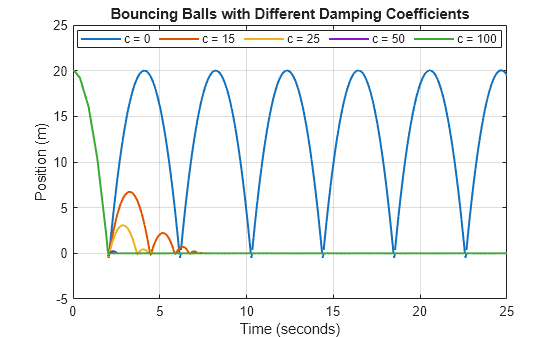
The results show the effect of varying the amount of damping in the system.
The simulation that sets
cto2shows the behavior of the system with the least damping. When the system is lightly damped, the number of times the ball bounces and the rebound height of each bounce is largest.As the value of
cincreases, the ball comes to rest sooner, and the rebound height of each bounce decays more steeply.
Create Phase Portrait to Visualize System States
To analyze a dynamic system, you can create a phase portrait. The phase portrait visualizes the way the states in the system vary together over time in the phase space, also known as the state space. By viewing the phase portrait of a system, you can easily analyze the stability of the system, identify equilibrium points that indicate steady-state operation, and observe dynamic behaviors, such as limit cycles.
The second-order model of the bouncing ball has two states: the position and the velocity of the ball. Create a phase portrait of the states in the bouncing ball model by plotting the position on the -axis and the velocity on the -axis. Use the quiver function to annotate the trajectory of each ball with an arrow that represents the direction in which the states evolve over time.
This example uses the custom function plotPhasePortraits to plot the phase portraits. To view the code for the function, open the file plotPhasePortraits.m using the edit function.
edit plotPhasePortraits.m
Plot the phase portraits using the plotPhasePortraits function.
phaselayout = plotPhasePortraits(pos,vel,cVector,N);
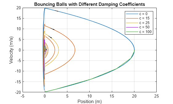
The trajectory of the ball from each simulation starts from the initial position and velocity and spirals inward to an equilibrium point at which the ball is at rest on the surface, with both a position and velocity of 0. As the damping coefficient increases, the ball reaches the equilibrium point faster, with fewer cycles in the spiral.
Postprocess Simulation Output
To further analyze the effect of the damping coefficient on the dynamics of the bouncing ball, you can extract more information by postprocessing the simulation results. This example postprocesses the simulation results using a custom function named analyzeResult. The function determines:
The number of times the ball bounces in each simulation.
The time of each collision between the ball and the surface.
To view the postprocessing code, open the file analyzeResult.m using the edit function.
edit("analyzeResult.m")
To postprocess the simulation results, call the function.
[numbounces, tcollision] = analyzeResult(out);
Analyze Effect of Damping on Number of Bounces
To see how the amount of damping in the model affects the number of times the ball bounces, plot the number of bounces against the value of the damping coefficient.
figure
plot(cVector,numbounces,"-o",MarkerEdgeColor="b",LineWidth=1);
grid on
title("Number of Bounces vs Damping Coefficient")
xlabel("Damping Coefficient (Ns/m)")
ylabel("Number of Bounces")
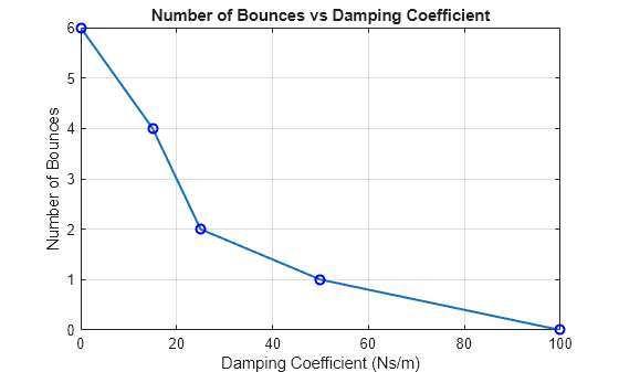
The plot confirms that the number of bounces decreases as the amount of damping in the system increases. When the damping coefficient is large enough, the ball does not bounce at all.
If you have a license for Curve Fitting Toolbox™, you can use the fit function to estimate the relationship between the damping coefficient and the number of bounces by fitting a curve to the data.
Analyze Bounce Timing
To understand how the damping coefficient affects the timing of each bounce, plot the time of each collision between the ball and the surface against the collision number. Because the ball with a damping coefficient of 64 does not bounce, the plot shows data for only five of the six simulated damping coefficients.
valididx = ~cellfun(@isempty,tcollision);
tcollision = tcollision(valididx);

for n = numel(tcollision):-1:1
    dispname = sprintf("c = %d",cVector(n));
    ncollision = 1:numel(tcollision{n});
    t = tcollision{n};
    h(n) = plot(ncollision,t,"-o",LineWidth=1,DisplayName=dispname);
    hold on
end

grid on
xlabel("Collision Number")
ylabel("Time of Collision (seconds)")
legend(h,Location="best")
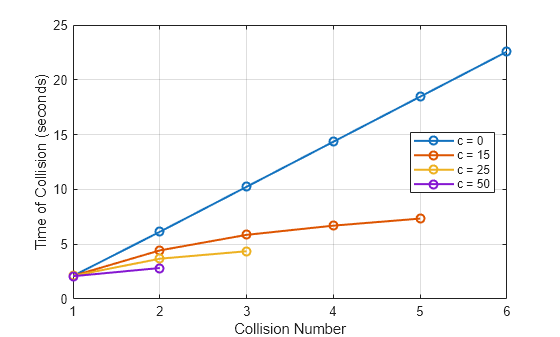
The nonlinearity in the restoring force affects the timing between bounces. When the system is lightly damped, the nonlinear term in the system equations contributes more to the overall system response. For small values of c, the relationship between the collision number and collision time is nonlinear.
As the damping coefficient value increases, the nonlinear term contributes less to the overall system response. For larger values of c, the relationship between the collision number and collision time appears more linear.
To further explore the effect of the nonlinearity in the restoring force, you can run additional simulations to analyze the impact of the model parameter .
Specify a single, scalar value for the damping coefficient .
Define a vector of values to simulate.
Create an array of
Simulink.SimulationInputobjects to configure each simulation in the parameter sweep. Use the vector of values to specify a different value of the variablealphaon eachSimulink.SimulationInputobject.Run the parameter sweep simulations using the array of
Simulink.SimulationInputobjects and repeat the analysis of the simulation results.