Main Content

Filter Analysis Using FVTool

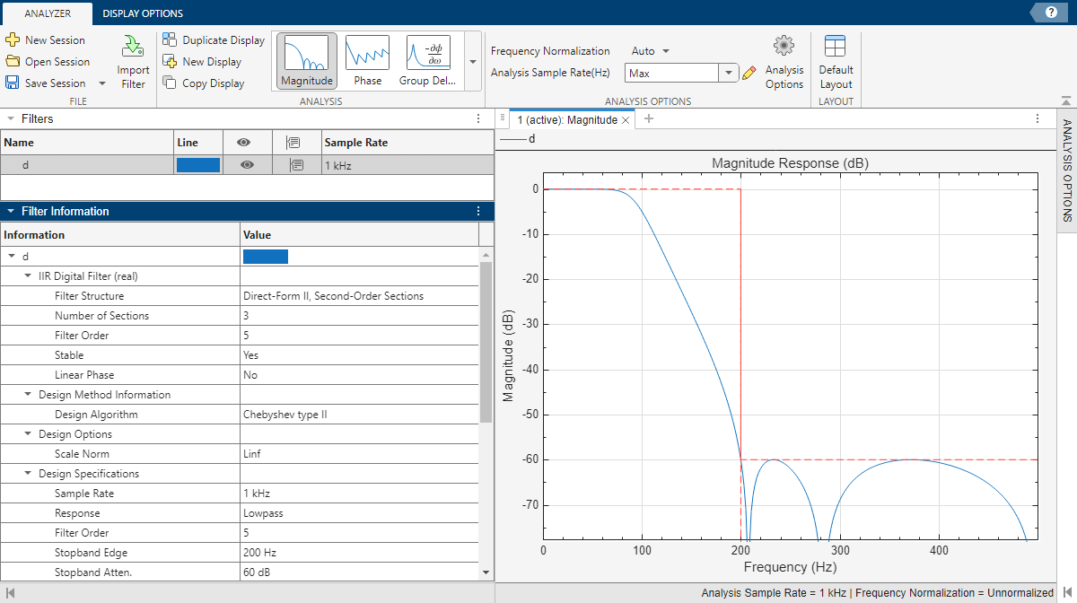
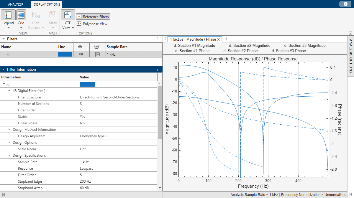
This example shows how to use several filter analysis functions in a single figure window by using the Filter Visualization Tool (FVTool), a graphical user interface available in Signal Processing Toolbox™.

FVTool also has an Application Program Interface (API) that allows you to interact with the GUI from the command line. This enables you to integrate FVTool into other applications.

Launch FVTool

We want to create a lowpass filter with a passband frequency of 0.4π rad/sample, a stopband frequency of 0.6π rad/sample, a passband ripple of 1 dB and a stopband attenuation of 80 dB. We design the filters using some of the Signal Processing Toolbox filter design tools and then analyze the results in FVTool.

Design a lowpass equiripple FIR filter.

Df1 = designfilt("lowpassfir",PassbandFrequency=0.4,...
                              StopbandFrequency=0.6,...
                              PassbandRipple=1,...
                              StopbandAttenuation=80,...
                              DesignMethod="equiripple");

Design a lowpass elliptic IIR filter.

Df2 = designfilt("lowpassiir",PassbandFrequency=0.4,...
                              StopbandFrequency=0.6,...
                              PassbandRipple=1,...
                              StopbandAttenuation=80,...
                              DesignMethod="ellip");

Launch FVTool with the filter objects and return a handle to FVTool which enables us to reuse the same FVTool figure.

hfvt = fvtool(Df1,Df2);

Add and Remove Filters

We can observe that both filters meet the design specifications, but we also want to see how well the Chebyshev Type II design performs.

You can add a filter to FVTool using the addfilter function.

Df3 = designfilt("lowpassiir",PassbandFrequency=0.4,...
                              StopbandFrequency=0.6,...
                              PassbandRipple=1,...
                              StopbandAttenuation=80,...
                              DesignMethod="cheby2");
addfilter(hfvt,Df3);

To identify which line on the plot belongs to which filter, you can add a legend using the legend function of the FVTool handle.

legend(hfvt,"Equiripple","Elliptic","Chebyshev Type II");

You can remove a filter from FVTool using the deletefilter function and passing the index of the filter(s) that you want to remove.

deletefilter(hfvt,[1 3]);

Change Analysis Parameters

The handle that FVTool returns contains properties that allow you to interact with both the filter and the current analysis. To see all of the available properties, use the get command. Display the last fourteen properties which are specific to FVTool.

s = get(hfvt);
% Keep the last 14 properties
c = struct2cell(s);
f = fieldnames(s);
s = cell2struct(c(end-14:end),f(end-14:end),1)
s = struct with fields:
       SelectionHighlight: on
                      Tag: 'filtervisualizationtool'
                 UserData: []
                  Visible: on
      NormalizedFrequency: 'on'
           FrequencyRange: '[0, pi)'
         MagnitudeDisplay: 'Magnitude (dB)'
          FrequencyVector: [0 0.0039 0.0078 0.0118 0.0157 0.0196 0.0235 0.0275 0.0314 0.0353 0.0392 0.0431 0.0471 0.0510 0.0549 0.0588 0.0627 0.0667 0.0706 0.0745 0.0784 0.0824 0.0863 0.0902 0.0941 0.0980 0.1020 0.1059 0.1098 0.1137 ... ] (1x256 double)
                 Analysis: 'magnitude'
        OverlayedAnalysis: ''
            PolyphaseView: 'off'
            ShowReference: 'on'
           FrequencyScale: 'Linear'
           NumberofPoints: 8192
    NormalizeMagnitudeto1: 'off'

All the parameters that are available from the FVTool Analysis Parameters dialog are also available as properties of the FVTool object. The set command with only two input arguments returns all possible values.

set(hfvt,"MagnitudeDisplay")
ans = 1x4 cell
    {'Magnitude'}    {'Magnitude (dB)'}    {'Magnitude squared'}    {'Zero-phase'}

Turn the display to Magnitude Squared.

hfvt.MagnitudeDisplay = "Magnitude Squared";

Get all possible values for the Analysis property.

set(hfvt,"Analysis")
ans = 1x12 cell
    {'magnitude'}    {'phase'}    {'freq'}    {'grpdelay'}    {'phasedelay'}    {'impulse'}    {'step'}    {'polezero'}    {'coefficients'}    {'info'}    {'magestimate'}    {'noisepower'}

Now change the analysis to look at the group delay response of the filter. Display the default units.

hfvt.Analysis = "grpdelay";
GroupDelayUnits = hfvt.GroupDelayUnits
GroupDelayUnits = 
'Samples'

Overlay Two Analyses

We would also like to see how the group delay and the magnitude response overlap in the frequency domain.

You can overlay any two analyses in FVTool that share a common x-axis (time or frequency) by setting the OverlayedAnalysis property.

set(hfvt,OverlayedAnalysis="magnitude",Legend="On")

To turn off the overlayed analysis, set the OverlayedAnalysis property to ''.

hfvt.OverlayedAnalysis = '';

You can close the FVTool figure by calling the close function on the FVTool handle.

close(hfvt)

See Also

Apps

Functions

Go to top of page