xwvd
Cross Wigner-Ville distribution and cross smoothed pseudo Wigner-Ville distribution
Syntax
Description
d = xwvd(___,"smoothedPseudo")x and
y. The function uses the length of the input signals to choose the
lengths of the windows used for time and frequency smoothing. This syntax can include any
combination of input arguments from previous syntaxes.
xwvd(___) with no output arguments plots the real
part of the cross Wigner-Ville or cross smoothed pseudo Wigner-Ville distribution in the
current figure.
Examples
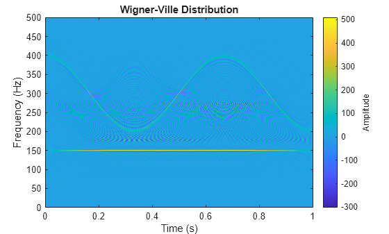
Generate two signals sampled at 1 kHz for 1 second and embedded in white noise. One signal is a sinusoid of frequency 150 Hz. The other signal is a chirp whose frequency varies sinusoidally between 200 Hz and 400 Hz. The noise has a variance of .
fs = 1000;
t = (0:1/fs:1)';

x = cos(2*pi*t*150) + 0.1*randn(size(t));
y = vco(cos(3*pi*t),[200 400],fs) + 0.1*randn(size(t));
Compute the Wigner-Ville distribution of the sum of the signals.
wvd(x+y,fs)
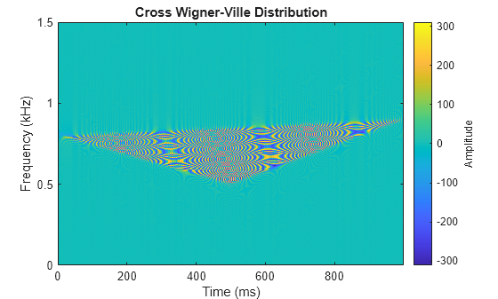
Compute and plot the cross Wigner-Ville distribution of the signals. The cross-distribution corresponds to the cross-terms of the Wigner-Ville distribution.
xwvd(x,y,fs)

Generate a two-channel signal that consists of two chirps. The signal is sampled at 3 kHz for one second. The first chirp has an initial frequency of 400 Hz and reaches 800 Hz at the end of the sampling. The second chirp starts at 500 Hz and reaches 1000 Hz at the end. The second chirp has twice the amplitude of the first chirp.
fs = 3000;
t = (0:1/fs:1-1/fs)';

x1 = chirp(t,1400,t(end),800);
x2 = 2*chirp(t,200,t(end),1000);
Store the signal as a timetable. Compute and plot the cross Wigner-Ville distribution of the two channels.
xt = timetable(seconds(t),x1,x2);

xwvd(xt(:,1),xt(:,2))
Compute the instantaneous frequency of a signal by using a known reference signal and the cross Wigner-Ville distribution.
Create a reference signal consisting of a Gaussian atom sampled at 1 kHz for 1 second. A Gaussian atom is a sinusoid modulated by a Gaussian. Specify a sinusoid frequency of 50 Hz. The Gaussian is centered at 64 milliseconds and has a variance of .
fs = 1e3;
t = (0:1/fs:1-1/fs)';

mu = 0.064;
sigma = 0.01;
fsin = 50;

xr = exp(-(t-mu).^2/(2*sigma^2)).*sin(2*pi*fsin*t);
Create the "unknown" signal to analyze, consisting of a chirp. The signal starts suddenly at 0.4 second and ends suddenly half a second later. In that lapse, the frequency of the chirp decreases linearly from 400 Hz to 100 Hz.
f0 = 400;
f1 = 100;

xa = zeros(size(t));
xa(t>0.4 & t<=0.9) = chirp((0:1/fs:0.5-1/fs)',f0,0.5,f1);
Create a two-component signal consisting of the sum of the unknown and reference signals. The smoothed pseudo Wigner-Ville distribution of the result provides an "ideal" time-frequency representation.
Compute and display the smoothed pseudo Wigner-Ville distribution.
w = wvd(xa+xr,fs,"smoothedPseudo");

wvd(xa+xr,fs,"smoothedPseudo")

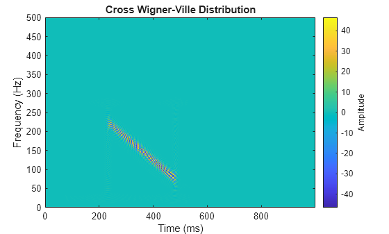
Compute the cross Wigner-Ville distribution of the unknown and reference signals. Take the absolute value of the distribution and set to zero the elements with amplitude less than 10. The cross Wigner-Ville distribution is equal to the cross-terms of the two-component signal.
Plot the real part of the cross Wigner-Ville distribution.
[c,fc,tc] = xwvd(xa,xr,fs);
c = abs(c);
c(c<10) = 0;

xwvd(xa,xr,fs)
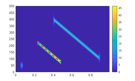
Enhance the Wigner-Ville cross-terms by adding the ideal time-frequency representation to the cross Wigner-Ville distribution. The cross-terms of the Wigner-Ville distribution occur halfway between the reference signal and the unknown signal.
d = w + c;

d = abs(real(d));

imagesc(tc,fc,d)
axis xy
colorbar
Identify and plot the high-energy ridge corresponding to the cross-terms. To isolate the ridge, find the time values where the cross-distribution has nonzero energy.
ff = tfridge(c,fc);

tv = sum(c)>0;

ff = ff(tv);
tc = tc(tv);

hold on
plot(tc,ff,"r--",linewidth=2)
hold off
Reconstruct the instantaneous frequency of the unknown signal by using the ridge and the reference function. Plot the instantaneous frequency as a function of time.
tEst = 2*tc - mu;
fEst = 2*ff - fsin;

plot(tEst,fEst)

Input Arguments
Output Arguments
More About
References
[1] Cohen, Leon. Time-Frequency Analysis: Theory and Applications. Englewood Cliffs, NJ: Prentice-Hall, 1995.
[2] Mallat, Stéphane. A Wavelet Tour of Signal Processing. Second Edition. San Diego, CA: Academic Press, 1999.
[3] Malnar, Damir, Victor Sucic, and Boualem Boashash. "A cross-terms geometry based method for components instantaneous frequency estimation using the cross Wigner-Ville distribution." In 11th International Conference on Information Sciences, Signal Processing and their Applications (ISSPA), pp. 1217–1222. Montréal: IEEE®, 2012.