invfreqs

Identify continuous-time filter parameters from frequency response data

Syntax

[b,a] = invfreqs(h,w,n,m)

[b,a] = invfreqs(h,w,n,m,wt)

[b,a] = invfreqs(___,iter)

[b,a] = invfreqs(___,tol)

[b,a] = invfreqs(___,'trace')

[b,a] = invfreqs(h,w,'complex',n,m,___)

Description

[b,a] = invfreqs(h,w,n,m) returns the real numerator and denominator coefficient vectors b and a of the transfer function h.

[b,a] = invfreqs(h,w,n,m,wt) weights the fit-errors versus frequency using wt.

[b,a] = invfreqs(___,iter) provides an algorithm that guarantees stability of the resulting linear system by searching for the best fit using a numerical, iterative scheme. This syntax can include any combination of input arguments from the previous syntaxes.

[b,a] = invfreqs(___,tol) uses tol to decide convergence of the iterative algorithm.

[b,a] = invfreqs(___,'trace') displays a textual progress report of the iteration.

[b,a] = invfreqs(h,w,'complex',n,m,___) creates a complex filter. In this case no symmetry is enforced, and the frequency is specified in radians between –π and π.

Examples

Transfer Function to Frequency Response Conversion

Convert a simple transfer function to frequency-response data and then back to the original filter coefficients.

a = [1 2 3 2 1 4];
b = [1 2 3 2 3];

[h,w] = freqs(b,a,64);
[bb,aa] = invfreqs(h,w,4,5)

bb = 1×5

    1.0000    2.0000    3.0000    2.0000    3.0000

aa = 1×6

    1.0000    2.0000    3.0000    2.0000    1.0000    4.0000

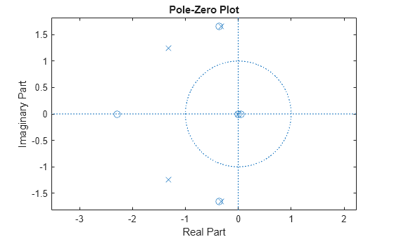
bb and aa are equivalent to b and a, respectively. However, the system is unstable because aa has poles with positive real part. View the poles of bb and aa.

zplane(bb,aa)

Use the iterative algorithm of invfreqs to find a stable approximation to the system.

[bbb,aaa] = invfreqs(h,w,4,5,[],30)

  INITIAL ESTIMATE
Current fit: 14.6322
par-vector
    2.0000
    3.0000
    2.0000
    1.0000
    4.0000
    1.0000
    2.0000
    3.0000
    2.0000
    3.0000

0
      ITERATION # 1
Current fit:  10.7257  Previous fit:  14.6322
Current par prev.par   GN-dir
    8.8120    2.0000   -6.8120
   22.6038    3.0000  -19.6038
   37.7456    2.0000  -35.7456
   30.7079    1.0000  -29.7079
   19.0754    4.0000  -15.0754
    0.8255    1.0000    0.1745
    9.2270    2.0000   -7.2270
   12.1247    3.0000   -9.1247
    9.0900    2.0000   -7.0900
   13.3229    3.0000  -10.3229

Norm of GN-vector: 1.02
0
1
      ITERATION # 2
Current fit:  5.2165  Previous fit:  10.7257
Current par prev.par   GN-dir
    6.3781    8.8120    4.8679
   14.6152   22.6038   15.9772
   19.6572   37.7456   36.1768
   15.6202   30.7079   30.1754
    6.1840   19.0754   25.7828
    0.8118    0.8255    0.0274
    5.5594    9.2270    7.3351
    5.0094   12.1247   14.2306
    9.4769    9.0900   -0.7739
    2.6124   13.3229   21.4211

Norm of GN-vector: 1.02
0
1
      ITERATION # 3
Current fit:  3.9314  Previous fit:  5.2165
Current par prev.par   GN-dir
    4.1801    6.3781    4.3960
    9.4121   14.6152   10.4062
    9.3775   19.6572   20.5594
    8.1148   15.6202   15.0109
    1.7929    6.1840    8.7822
    0.8191    0.8118   -0.0146
    2.9779    5.5594    5.1629
    3.9421    5.0094    2.1345
    3.7840    9.4769   11.3860
    0.9825    2.6124    3.2598

Norm of GN-vector: 1.02
0
1
      ITERATION # 4
Current fit:  3.76  Previous fit:  3.9314
Current par prev.par   GN-dir
    3.1641    4.1801    2.0320
    8.0369    9.4121    2.7504
   11.6674    9.3775   -4.5798
    8.5321    8.1148   -0.8347
    5.7079    1.7929   -7.8301
    0.8245    0.8191   -0.0107
    1.8347    2.9779    2.2865
    4.8827    3.9421   -1.8811
    3.4502    3.7840    0.6675
    3.0012    0.9825   -4.0375

Norm of GN-vector: 1.02
0
      ITERATION # 5
Current fit:  3.6897  Previous fit:  3.76
Current par prev.par   GN-dir
    5.5414    3.1641   -2.3773
   13.6887    8.0369   -5.6518
   22.3820   11.6674  -10.7146
   16.9016    8.5321   -8.3694
   12.6568    5.7079   -6.9489
    0.8463    0.8245   -0.0219
    3.6662    1.8347   -1.8316
    8.5813    4.8827   -3.6986
    6.9118    3.4502   -3.4616
    6.6495    3.0012   -3.6483

Norm of GN-vector: 1.02
0
      ITERATION # 6
Current fit:  3.6703  Previous fit:  3.6897
Current par prev.par   GN-dir
    9.7416    5.5414   -4.2002
   23.0042   13.6887   -9.3155
   40.1756   22.3820  -17.7936
   35.4599   16.9016  -18.5584
   28.1668   12.6568  -15.5099
    0.8137    0.8463    0.0326
    7.1751    3.6662   -3.5089
   13.5489    8.5813   -4.9676
   14.5313    6.9118   -7.6196
   14.8048    6.6495   -8.1553

Norm of GN-vector: 1.02
0
      ITERATION # 7
Current fit:  3.6657  Previous fit:  3.6703
Current par prev.par   GN-dir
   18.1583    9.7416   -8.4167
   47.0850   23.0042  -24.0808
   87.6701   40.1756  -47.4945
   85.6959   35.4599  -50.2360
   59.2754   28.1668  -31.1087
    0.7515    0.8137    0.0622
   14.1169    7.1751   -6.9418
   27.9647   13.5489  -14.4158
   36.5138   14.5313  -21.9825
   31.1937   14.8048  -16.3890

Norm of GN-vector: 1.02
0
1
2
3
4
      ITERATION # 8
Current fit:  3.6643  Previous fit:  3.6657
Current par prev.par   GN-dir
   10.2150   18.1583  127.0934
   26.2877   47.0850  332.7554
   46.2217   87.6701  663.1737
   45.2631   85.6959  646.9253
   26.6968   59.2754  521.2579
    0.7618    0.7515   -0.1648
    7.8062   14.1169  100.9715
   14.9328   27.9647  208.5090
   20.0396   36.5138  263.5861
   14.0374   31.1937  274.5012

Norm of GN-vector: 1.02
0
1
2
3
      ITERATION # 9
Current fit:  3.6529  Previous fit:  3.6643
Current par prev.par   GN-dir
    5.0286   10.2150   41.4913
   12.5896   26.2877  109.5850
   18.6943   46.2217  220.2194
   17.9670   45.2631  218.3684
    4.6265   26.6968  176.5620
    0.7690    0.7618   -0.0574
    3.6842    7.8062   32.9759
    6.3394   14.9328   68.7475
    8.9539   20.0396   88.6861
    2.4072   14.0374   93.0420

Norm of GN-vector: 1.02
0
1
2
3
4
      ITERATION # 10
Current fit:  3.6112  Previous fit:  3.6529
Current par prev.par   GN-dir
    3.9318    5.0286   17.5494
    9.4738   12.5896   49.8531
   12.5970   18.6943   97.5578
   11.7310   17.9670   99.7758
    0.8446    4.6265   60.5104
    0.7733    0.7690   -0.0690
    2.7882    3.6842   14.3365
    4.4477    6.3394   30.2677
    6.1980    8.9539   44.0935
    0.4156    2.4072   31.8644

Norm of GN-vector: 1.02
0
1
2
3
4
5
      ITERATION # 11
Current fit:  3.5702  Previous fit:  3.6112
Current par prev.par   GN-dir
    3.6840    3.9318    7.9300
    8.7625    9.4738   22.7603
   11.2344   12.5970   43.6021
   10.3776   11.7310   43.3107
    0.1619    0.8446   21.8471
    0.7716    0.7733    0.0556
    2.5818    2.7882    6.6028
    4.0067    4.4477   14.1117
    5.5630    6.1980   20.3217
    0.0515    0.4156   11.6522

Norm of GN-vector: 1.02
0
1
2
3
4
5
6
      ITERATION # 12
Current fit:  3.3656  Previous fit:  3.5702
Current par prev.par   GN-dir
    3.6207    3.6840    5.1581
    8.6043    8.7625   14.1438
   10.9485   11.2344   27.8311
   10.1562   10.3776   26.2605
    0.0874    0.1619   15.9587
    0.7689    0.7716    0.1701
    2.5150    2.5818    4.2758
    3.8562    4.0067    9.6304
    5.3710    5.5630   12.2833
   -0.0846    0.0515    8.7095

Norm of GN-vector: 1.02
0
1
2
3
4
5
      ITERATION # 13
Current fit:  3.2971  Previous fit:  3.3656
Current par prev.par   GN-dir
    3.5160    3.6207    3.6489
    8.3584    8.6043    8.9094
   10.5209   10.9485   16.1543
    9.8789   10.1562   11.9799
    0.0455    0.0874    4.2535
    0.7632    0.7689    0.1844
    2.4193    2.5150    3.0625
    3.6661    3.8562    6.0838
    5.1617    5.3710    6.7005
   -0.1544   -0.0846    2.2337

Norm of GN-vector: 1.02
0
1
2
3
4
5
      ITERATION # 14
Current fit:  3.2835  Previous fit:  3.2971
Current par prev.par   GN-dir
    3.4280    3.5160    3.1299
    8.1605    8.3584    7.4079
   10.1831   10.5209   13.3650
    9.6875    9.8789    9.3076
    0.0473    0.0455    2.9685
    0.7574    0.7632    0.1857
    2.3376    2.4193    2.6148
    3.5062    3.6661    5.1152
    4.9937    5.1617    5.3757
   -0.2007   -0.1544    1.4830

Norm of GN-vector: 1.02
0
1
2
3
4
5
      ITERATION # 15
Current fit:  3.2768  Previous fit:  3.2835
Current par prev.par   GN-dir
    3.3452    3.4280    2.8050
    7.9718    8.1605    6.5651
    9.8532   10.1831   11.8133
    9.4834    9.6875    8.0821
    0.0233    0.0473    2.2586
    0.7519    0.7574    0.1756
    2.2648    2.3376    2.3317
    3.3661    3.5062    4.4856
    4.8466    4.9937    4.7069
   -0.2326   -0.2007    1.0209

Norm of GN-vector: 1.02
0
1
2
3
4
5
6
      ITERATION # 16
Current fit:  3.2708  Previous fit:  3.2768
Current par prev.par   GN-dir
    3.3076    3.3452    2.5149
    7.8868    7.9718    5.7924
    9.7025    9.8532   10.4860
    9.3897    9.4834    7.0322
    0.0078    0.0233    1.9923
    0.7492    0.7519    0.1734
    2.2323    2.2648    2.0796
    3.3036    3.3661    3.9950
    4.7821    4.8466    4.1235
   -0.2462   -0.2326    0.8669

Norm of GN-vector: 1.02
0
1
2
3
4
5
6
7
8
      ITERATION # 17
Current fit:  3.2656  Previous fit:  3.2708
Current par prev.par   GN-dir
    3.2983    3.3076    2.3862
    7.8655    7.8868    5.4429
    9.6639    9.7025    9.8950
    9.3641    9.3897    6.5518
    0.0004    0.0078    1.9112
    0.7485    0.7492    0.1736
    2.2246    2.2323    1.9679
    3.2889    3.3036    3.7864
    4.7671    4.7821    3.8599
   -0.2494   -0.2462    0.8281

Norm of GN-vector: 1.02
0
1
2
3
4
5
6
7
8
9
10
11
12
13
14
15
16
17
18
19
      ITERATION # 18
Current fit:  3.2656  Previous fit:  3.2656
Current par prev.par   GN-dir
    3.2983    3.2983   -0.0232
    7.8655    7.8655   -0.0177
    9.6639    9.6639   -0.0221
    9.3641    9.3641    0.0585
    0.0004    0.0004    0.3879
    0.7485    0.7485    0.0384
    2.2246    2.2246    0.0541
    3.2889    3.2889    0.0536
    4.7671    4.7671   -0.1003
   -0.2494   -0.2494   -0.1377

Norm of GN-vector: 1.02
No improvement of the criterion possible along the search direction
Iterations therefore terminated

bbb = 1×5

    0.7485    2.2246    3.2889    4.7671   -0.2494

aaa = 1×6

    1.0000    3.2983    7.8655    9.6639    9.3641    0.0004

Verify that the system is stable by plotting the new poles.

zplane(bbb,aaa)

Continuous-Time Transfer Function

Generate two vectors, mag and phase, that simulate magnitude and phase data gathered in a laboratory. Also generate a vector, w, of frequencies.

rng('default')

fs = 1000;
t = 0:1/fs:2;
mag = periodogram(sin(2*pi*100*t)+randn(size(t))/10,[],[],fs);
phase = randn(size(mag))/10;
w = linspace(0,fs/2,length(mag))';

Use invfreqs to convert the data into a continuous-time transfer function. Plot the result.

[b,a] = invfreqs(mag.*exp(1j*phase),w,2,2,[],4);

  INITIAL ESTIMATE
Current fit: 0.94648
par-vector
   1.0e+04 *

    0.0000
    1.0019
    0.0000
   -0.0000
    0.0000

0
      ITERATION # 1
Current fit:  0.88173  Previous fit:  0.94648
Current par prev.par   GN-dir
   1.0e+04 *

    0.0000    0.0000    0.0000
    0.9997    1.0019    0.0022
    0.0000    0.0000   -0.0000
    0.0000   -0.0000   -0.0000
    0.0003    0.0000   -0.0003

Norm of GN-vector: 1.02
0
      ITERATION # 2
Current fit:  0.75065  Previous fit:  0.88173
Current par prev.par   GN-dir
   1.0e+03 *

    0.0015    0.0000   -0.0015
    9.8048    9.9974    0.1926
    0.0000    0.0000    0.0000
    0.0000    0.0000   -0.0000
    0.0001    0.0032    0.0031

Norm of GN-vector: 1.02
0
1
      ITERATION # 3
Current fit:  0.74495  Previous fit:  0.75065
Current par prev.par   GN-dir
   1.0e+04 *

    0.0013    0.0002   -0.0024
    1.0245    0.9805   -0.0880
    0.0000    0.0000   -0.0000
    0.0000    0.0000   -0.0000
   -0.0003    0.0000    0.0006

Norm of GN-vector: 1.02
0
1
2
3
      ITERATION # 4
Current fit:  0.73558  Previous fit:  0.74495
Current par prev.par   GN-dir
   1.0e+04 *

    0.0008    0.0013    0.0039
    0.9760    1.0245    0.3878
    0.0000    0.0000   -0.0000
    0.0000    0.0000    0.0000
   -0.0002   -0.0003   -0.0003

Norm of GN-vector: 1.02

freqs(b,a)

Input Arguments

h — Frequency response

vector

Frequency response, specified as a vector.

w — Angular frequencies

vector

Angular frequencies at which h is computed, specified as a vector.

n, m — Desired order

positive integer scalar

Desired order of the numerator and denominator polynomials, specified as positive integer scalars.

Data Types: single | double

wt — Weighting factors

vector

Weighting factors, specified as a vector. wt is a vector of weighting factors that is the same length as w.

Data Types: single | double

iter — Number of iterations in the search algorithm

positive real scalar

Number of iterations in the search algorithm, specified as a positive real scalar. The iter parameter tells invfreqs to end the iteration when the algorithm has converged to a solution, or after iter iterations, whichever occurs first.

tol — Tolerance

0.01 (default) | scalar

Tolerance, specified as a scalar. invfreqs defines convergence as occurring when the norm of the (modified) gradient vector is less than tol.

To obtain a weight vector of all ones, use

invfreqs(h,w,n,m,[],iter,tol)

Output Arguments

b, a — Transfer function coefficients

vectors

Transfer function coefficients, returned as vectors. Express the transfer function in terms of b and a as

$$H(s)=\frac{B(s)}{A(s)}=\frac{b(1)s^n+b(2)s^{n-1}+\cdots +b(n+1)}{a(1)s^m+a(2)s^{m-1}+\cdots +a(m+1)}$$

Example: b = [1 3 3 1]/6 and a = [3 0 1 0]/3 specify a third-order Butterworth filter with normalized 3 dB frequency 0.5π rad/sample.

Data Types: double | single
Complex Number Support: Yes

Tips

When building higher order models using high frequencies, it is important to scale the frequencies, dividing by a factor such as half the highest frequency present in w, so as to obtain well-conditioned values of a and b. This corresponds to a rescaling of time.

Algorithms

By default, invfreqs uses an equation error method to identify the best model from the data. This finds b and a in

$$\underset{b,a}{\min }{\displaystyle \sum _{k=1}^{n}wt(k){\left|h(k)A(w(k))-B(w(k))\right|}^2}$$

by creating a system of linear equations and solving them with the MATLAB^® \ operator. Here A(w(k)) and B(w(k)) are the Fourier transforms of the polynomials a and b, respectively, at the frequency w(k), and n is the number of frequency points (the length of h and w). This algorithm is based on Levi [1]. Several variants have been suggested in the literature, where the weighting function wt gives less attention to high frequencies.

The superior (“output-error”) algorithm uses the damped Gauss-Newton method for iterative search [2], with the output of the first algorithm as the initial estimate. This solves the direct problem of minimizing the weighted sum of the squared error between the actual and the desired frequency response points.

$$\underset{b,a}{\min }{\displaystyle \sum _{k=1}^{n}wt(k){\left|h(k)-\frac{B(w(k))}{A(w(k))}\right|}^2}$$

References

[1] Levi, E. C. “Complex-Curve Fitting.” IRE Trans. on Automatic Control. Vol. AC-4, 1959, pp. 37–44.

[2] Dennis, J. E., Jr., and R. B. Schnabel. Numerical Methods for Unconstrained Optimization and Nonlinear Equations. Englewood Cliffs, NJ: Prentice-Hall, 1983.

Extended Capabilities

C/C++ Code Generation
Generate C and C++ code using MATLAB® Coder™.

Version History

Introduced before R2006a

R2024b: invfreqs supports C/C++ code generation

The invfreqs function supports C/C++ code generation. You must have MATLAB Coder™ to use this functionality.