Main Content

ctf2zp

Convert cascaded transfer functions to zero-pole-gain form

Since R2024b

    Description

    [z,p] = ctf2zp(B,A) computes the zeros z and poles p of a system represented as Cascaded Transfer Functions (CTF) with numerator coefficients B and denominator coefficients A.

    example

    [z,p] = ctf2zp(B,A,g) specifies the scale values, g, across filter sections.

    [___,k] = ctf2zp(___) returns the scalar gain k of the system. Use this syntax with any of the input or output arguments in previous syntaxes.

    example

    Examples

    collapse all

    Specify a two-section digital filter with a transfer function H(z) in the CTF format. Plot the 1024-point frequency response of the filter.

    H(z)=(0.1607+0.2414z-1+0.4689z-2)×0.1607+0.0828z-1+0.0551z-21-1.1940z-1+0.4360z-2

    B = [0.1607    0.2414    0.4689
         0.1607    0.0828    0.0551];
    A = [     1         0         0;
              1   -1.1940    0.4360];
    freqz(B,A,1024,"ctf")

    Figure contains 2 axes objects. Axes object 1 with title Phase, xlabel Normalized Frequency (\times\pi rad/sample), ylabel Phase (degrees) contains an object of type line. Axes object 2 with title Magnitude, xlabel Normalized Frequency (\times\pi rad/sample), ylabel Magnitude (dB) contains an object of type line.

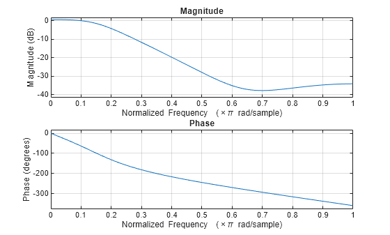
    Compute the zeros and poles of the transfer function.

    [z,p] = ctf2zp(B,A)
    z = 4×1 complex
    
      -0.7511 + 1.5342i
      -0.7511 - 1.5342i
      -0.2576 + 0.5258i
      -0.2576 - 0.5258i
    
    
    p = 4×1 complex
    
       0.0000 + 0.0000i
       0.0000 + 0.0000i
       0.5970 + 0.2821i
       0.5970 - 0.2821i


    Create a 10th-order bandpass digital elliptic filter in the CTF form.

    [B,A,gS] = ellip(10,0.1,60,[0.35 0.65],"ctf")
    B = 5×5
    
        1.0000   -0.0000   -1.3205    0.0000    1.0000
        1.0000    0.0000    0.3308   -0.0000    1.0000
        1.0000   -0.0000    0.8670   -0.0000    1.0000
        1.0000    0.0000    1.0340    0.0000    1.0000
        1.0000    0.0000    1.0853   -0.0000    1.0000
    
    
    A = 5×5
    
        1.0000   -0.0000    1.2677   -0.0000    0.4407
        1.0000    0.0000    1.2212    0.0000    0.6374
        1.0000   -0.0000    1.1779   -0.0000    0.8251
        1.0000    0.0000    1.1571    0.0000    0.9300
        1.0000   -0.0000    1.1561   -0.0000    0.9818
    
    
    gS = 
    0.0053
    

    Specify scale values. Because the filter has five fourth-order sections, the vector of scale values must have six elements.

    g = [1:size(B,1) gS]
    g = 1×6
    
        1.0000    2.0000    3.0000    4.0000    5.0000    0.0053


    Get the zero-pole decomposition of the filter. Plot the zeros and poles in the z-plane.

    [z,p,k] = ctf2zp(B,A,g);
    zplane(z,p)
    title("Pole-Zero Plot, k = "+k)
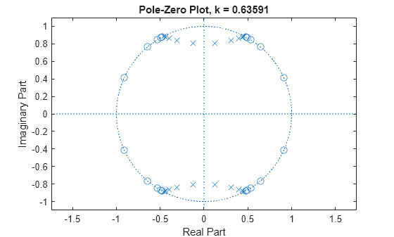
    Figure contains an axes object. The axes object with title Pole-Zero Plot, k = 0.63591, xlabel Real Part, ylabel Imaginary Part contains 3 objects of type line. One or more of the lines displays its values using only markers

    Input Arguments

    collapse all

    Since R2024b

    Cascaded transfer function (CTF) coefficients, specified as scalars, vectors, or matrices. B and A list the numerator and denominator coefficients of the cascaded transfer function, respectively.

    B must be of size L-by-(m + 1) and A must be of size L-by-(n + 1), where:

    • L represents the number of filter sections.

    • m represents the order of the filter numerators.

    • n represents the order of the filter denominators.

    For more information about the cascaded transfer function format and coefficient matrices, see Specify Digital Filters in CTF Format.

    Note

    If any element of A(:,1) is not equal to 1, then ctf2zp normalizes the filter coefficients by A(:,1). In this case, A(:,1) must be nonzero.

    Data Types: double | single
    Complex Number Support: Yes

    Since R2024b

    Scale values, specified as a real-valued scalar or as a real-valued vector with L + 1 elements, where L is the number of CTF sections. The scale values represent the distribution of the filter gain across the sections of the cascaded filter representation.

    The ctf2zp function applies a gain to the filter sections using the scaleFilterSections function depending on how you specify g:

    • Scalar — The function distributes the gain uniformly across all filter sections.

    • Vector — The function applies the first L gain values to the corresponding filter sections and distributes the last gain value uniformly across all filter sections.

    Data Types: double | single

    Output Arguments

    collapse all

    System zeros and poles, returned as column vectors.

    The vectors z and p contain the n zeros and m poles of the transfer function H(z), respectively.

    H(z)=k(zz1)(zz2)(zzn)(zp1)(zp2)(zpm).

    System gain, returned as a scalar.

    The scalar k represents the gain of the transfer function H(z).

    H(z)=k(zz1)(zz2)(zzn)(zp1)(zp2)(zpm).

    More About

    collapse all

    Tips

    • You can obtain filters in CTF format, including the scaling gain. Use the outputs of digital IIR filter design functions, such as butter, cheby1, cheby2, and ellip. Specify the "ctf" filter-type argument in these functions and specify to return B, A, and g to get the scale values. (since R2024b)

    References

    [1] Lyons, Richard G. Understanding Digital Signal Processing. Upper Saddle River, NJ: Prentice Hall, 2004.

    Extended Capabilities

    expand all

    C/C++ Code Generation
    Generate C and C++ code using MATLAB® Coder™.

    Version History

    Introduced in R2024b

    See Also

    Apps

    Functions