The SerDes Toolbox DFE Adaptation
The SerDes Toolbox Decision Feedback Equalizer (DFE) adaptation is a "blind" correlation-based adaptive equalization algorithm. Equalizers compensate for loss and reflections in wired communication systems and adaptive algorithms can determine in real time the best equalization setting to use. All adaptive algorithms determine the distance (or error) between the actual and desired behavior and then work to reduce this error. Some algorithms use a training sequence, where a known pattern is sent through the system and the receiver then can directly calculate the error. A "blind" algorithm does not depend on a pre-arranged signal being sent but instead relies on assumptions about the data being sent. The assumption behind the adaptation algorithm in the SerDes Toolbox DFECDR System Object is that any correlation between the sampled waveform voltage and prior recovered symbols is due to inter-symbol interference (ISI) alone. This assumption is appropriate if the incoming data pattern is random.
This document illustrates the SerDes Toolbox DFE adaptation algorithm with the aim of educating its users to its features and limitations. The serdes.DFECDR is a white-box System object written in MATLAB and is open for inspection by users of the SerDes Toolbox. The following image is from the serdes.DFECDR system object and shows the section of code where the DFE tap weights are determined in sample-by-sample simulation mode.

There are two perspectives on the DFE tap and adaptation, each from a different simulation modality. The first is from LTI impulse response-based simulation (Init in AMI modeling language) where the ideal DFE tap weights can be directly read from the pulse response at 1, 2, . . . N symbols from the cursor sampling location. The second perspective is the time domain sample-by-sample simulation mode (GetWave in AMI modeling language) which is most similar to actual circuit behavior. Where with a typical simulation flow, the DFE taps are read from the pulse response, in this example when channel loss is set to zero, we artificially modify the pulse response to have a known amount of inter-symbol interference (ISI). This will allow us to validate the time domain DFE adaptation behavior when the tap value converge to the known ISI value. Note that as the DFE compensates for the ISI, the DFE tap weights are equal in magnitude to the ISI voltage and opposite in sign.
First define the system and study parameters:
SymbolTime = 100e-12;   %Time duration of a symbol
SamplesPerSymbol = 16;  %Over sampling factor

%If Loss = 0, then modify ideal pulse response with known amount of ISI
ISIvalue = 0.1;    %Artificial amount of ISI to add to the ideal channel
Loss = 0;          %Loss of channel (set to non-zero values for further exploration).

NTaps = 2;              %Number of DFE taps
StepSize = 0.0025;      %Adaptation step size
Order = 9;              %PRBS pattern order
NumberOfSymbols = 10000;%Number of symbols in pattern
Next, create a channel model and determine the receiver input impulse and pulse responses.
%Create channel Model at the specified loss
SampleInterval = SymbolTime/SamplesPerSymbol;   %Sample interval
FundamentalFrequency = 1/SymbolTime/2;          %Fundamental frequency
channelModel = serdes.ChannelLoss(...
    'Loss',Loss,...                 %Loss at target frequency
    'dt',SampleInterval,...         %Sample interval
    'TargetFrequency', FundamentalFrequency,... %Frequency for desired loss
    'TxR',50,'TxC',1e-14,...        %Near ideal Transmitter termination
    'RxR',50,'RxC',1e-14);          %Near ideal Receiver termination
Impulse = channelModel.impulse;

%Add ISI to the ideal pulse response
if Loss==0
    Impulse = Impulse + ISIvalue*circshift(Impulse,SamplesPerSymbol);
end

%Get pulse response
Pulse = impulse2pulse(Impulse,SamplesPerSymbol,SampleInterval);

%Determine pulse response clock recovery position with hula-hoop algorithm
ClockPositionIndex = round(pulseRecoverClock(Pulse,SamplesPerSymbol)) + SamplesPerSymbol*(0:NTaps);

%Visualize
TimeVector1 = SampleInterval*(0:length(Pulse)-1)/SymbolTime;
figure
plot(TimeVector1,Pulse,...
    TimeVector1(ClockPositionIndex(1)),Pulse(ClockPositionIndex(1)),'o',...
    TimeVector1(ClockPositionIndex(2:end)),Pulse(ClockPositionIndex(2:end)),'s')
xlabel('UI')
ylabel('voltage')
title('System Pulse Response')
axis([TimeVector1(ClockPositionIndex(1))-2,TimeVector1(ClockPositionIndex(1))+NTaps*1.5,...
    min(Pulse)-0.05,max(Pulse)+0.05])
grid on
legend('pulse','cursor','post-cursor ISI','location','best')

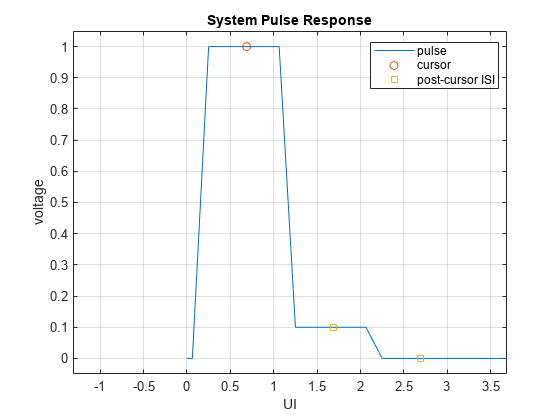
In the figure above, the pulse response and the sample locations for the cursor and post-cursor ISI are identified. A key point is that the DFE equalization will attempt to compensate for this post-cursor ISI. The ideal DFE tap value is equal in magnitude and opposite in sign of the pulse response at post-cursor positions. In sample-by-sample operation, the pulse response isn't available and explaining how the adaptation determines the DFE tap from one sample per symbol is the objective of this document.
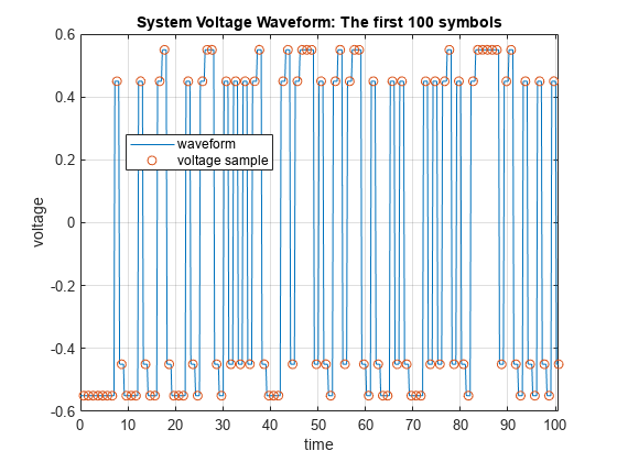
Our next step is to create a NRZ differential data pattern waveform from the pulse response. Then with the waveform we emulate a clock recovery circuit and extract the data voltage samples.
%Generate PRBS pattern
DataPattern = prbs(Order,NumberOfSymbols)-0.5;

%Combine pulse response with data pattern.
Wave = pulse2wave(Pulse,DataPattern,SamplesPerSymbol);

%Determine data sample position of waveform.  Normally, an adaptive CDR
%would be used but for simplicity we utilize the pulse response to
%determine the clock location.
WaveClockIndex = mod(ClockPositionIndex(1),SamplesPerSymbol):SamplesPerSymbol:(NumberOfSymbols*SamplesPerSymbol);

%Sample waveform voltage at clock positions
VoltageSample = Wave(WaveClockIndex);

figure
TimeVector2 = SampleInterval*(0:length(Wave)-1)/SymbolTime;
plot(TimeVector2,Wave,...
    TimeVector2(WaveClockIndex),VoltageSample,'o')
xlabel('time')
ylabel('voltage')
nsymbols = min(100,NumberOfSymbols);
title(sprintf('System Voltage Waveform: The first %g symbols',nsymbols))
grid on
ax = axis;
axis([0,TimeVector2(ClockPositionIndex(1))+nsymbols,ax(3:4)])
legend('waveform','voltage sample','location','best')

Now that we have the sampled voltages, we can simulate how the DFE adaptation algorithm will utilize them. The process is to first apply the DFE tap to the waveform, then determine the symbol (or recover the data) from the equalized voltages and then adapt the DFE tap values. Since this is a synthetic example, we can compare the adapted DFE taps to the ideal DFE tap values extracted from the pulse response.
Data = zeros(NumberOfSymbols,1);%data decision
VoltageSampleEQ = VoltageSample;%initialize equalized voltage samples vector
Weights = zeros(NTaps,1);       %tap weights
WeightsHistory = zeros(NumberOfSymbols,NTaps); %tap weight history

%Loop over symbols
for ii = NTaps+1:NumberOfSymbols

    %Apply DFE
    for kk = 1:NTaps
        %From serdes.DFECDR.m:
        %waveOut = waveOut + obj.DFEtapRounded(kk)*obj.SymbolShiftRegister(kk);
        VoltageSampleEQ(ii) = VoltageSampleEQ(ii) + Weights(kk)*Data(ii-kk);
    end

    %Determine Symbol.  Note that a symbol set of [-1/2,1/2] is easier to
    %work with mathematically than [0, 1]
    Data(ii) = sign(VoltageSampleEQ(ii))/2;

    %Adapt DFE
    for kk = 1:NTaps
        %From serdes.DFECDR.m:
        %obj.DFEtapInternal(kk) = obj.DFEtapInternal(kk) ...
        %                        - obj.EqualizationGain*obj.DataVoltage*obj.SymbolShiftRegister(kk);
        Weights(kk) = Weights(kk) - StepSize*VoltageSampleEQ(ii)*Data(ii-kk);
    end
    WeightsHistory(ii,:) = Weights;
end

%Determine the ideal tap weight from the pulse response for visualization
WeightsIdeal = -Pulse(ClockPositionIndex(2:end));

%visualize
figure
SymbolVector1 = 1:NumberOfSymbols;
plot(SymbolVector1,WeightsHistory,...
    [SymbolVector1(1),SymbolVector1(end)],[1;1]*WeightsIdeal','--'), grid on
ylabel('tap voltage')
xlabel('# of symbols')
title('DFE tap adaptation')
tapString = num2str((1:NTaps)');
legendStr = cellstr([[repmat('adapt ',NTaps,1),tapString];...
    [repmat('ideal ',NTaps,1),tapString]]);
legend(legendStr,'location','best')

You can observe from this figure, that this DFE algorithm is searching for a correlation between the prior data decision and the current equalized voltage sample. If the data pattern is truly random, then any correlation between the prior data decision, d[n-1]), and the current equalized voltage sample, v[n], will be due to ISI alone. Therefore, by accumulating this correlation, the DFE tap weights are determined. This is expressed below for the th tap weight, , that is found from accumulating the correlation between the time-shifted recovered data symbol sequence, , and the equalized voltage, , scaled by the stepsize factor .
See Appendix A for an informal derivation of the above equation.
"Blind" adaptation algorithms are attractive because they can directly operate on the signal of interest without requiring a training pattern. Additionally, "blind" adaptation has the advantage of being always active so to be able to compensate for factors such as temperature drift of the circuits.
There are other factors to consider, for instance a larger stepsize will result in faster convergence of the DFE tap weights. But a larger stepsize will have larger steady state variance around the ideal tap weight value. Therefore, some implementations scale the step size after convergence to try to get the advantages of both large and small step sizes.
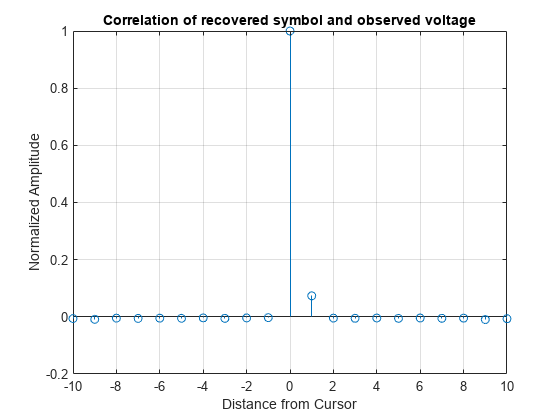
In this example, you can see it has been set up such that all of the symbol decisions and sampled voltages are recorded in a vector. Therefore, it is very straightforward to calculate the correlation between the recovered data and the voltage samples.
%Select a two repetitions of the PRBS pattern
PatternSelect = (1:min(2*(2^Order-1),NumberOfSymbols))+NTaps;

%Perform correlation
[CrossCorrelation,Lags] = xcorr(flipud(Data(PatternSelect)),flipud(VoltageSampleEQ(PatternSelect)));

%Determine index of cursor
CursorIndex = find(Lags==0);

%Normalize correlation
CrossCorrelationNormalized = CrossCorrelation/CrossCorrelation(CursorIndex);

%visualize
figure
stem(Lags,CrossCorrelationNormalized);
grid on
xlabel('Distance from Cursor')
ylabel('Normalized Amplitude')
title('Correlation of recovered symbol and observed voltage')
ax = axis;
axis([NTaps*5*[-1,1],ax(3:4)]),

For a Loss of 0 dB, it is satisfying to see that the correlation is evident from the vector correlation and even the magnitude of the correlation is similar to the injected amount of ISI.
Of course, an actual analog SerDes DFE won't be able to do a full vector correlation to determine the tap weights, therefore the same operation needs to be approximated in an iterative fashion. The code below shows how the first DFE tap correlation is performed in a sample-by-sample manner by multiplying the prior recovered symbol value and the current equalized waveform voltage. When this product is accumulated, the result is the DFE tap voltage.
%Perform multiplication between resolved data values and the equalized
%waveform.
DataTimesVoltageSampleEQ = Data(1:end-1).*VoltageSampleEQ(2:end);

%Visualize product
figure
SymbolVector2 = 2:NumberOfSymbols;
plot(SymbolVector2,DataTimesVoltageSampleEQ,'s')
legend('data[n-1] * vsampleEQ[n]','location','best')
grid on
xlabel('sample #')
title(sprintf('Product of previous recovered symbol and the equalized voltage sample'))
![Figure contains an axes object. The axes object with title Product of previous recovered symbol and the equalized voltage sample, xlabel sample # contains a line object which displays its values using only markers. This object represents data[n-1] * vsampleEQ[n].](../../examples/serdes/win64/DFEAdaptationExample_06.png)
Note how this product produces two trend lines, one positive and one negative. At the beginning the upper line is around 0.275 and the lower line is around -0.22, if there were no correlation, then the two lines would be opposite in sign and equal in magnitude. When the product is accumulated or added up, this difference in magnitude collects into the DFE tap weight. In this situation, as the DFE tap weight increases, the correlation between the sampled equalized waveform and the prior data symbol is reduced until the DFE tap value doesn't update much anymore. The DFE tap value has now converged to its final value. The following piece of code shows the cumulative sum of the product and how the resulting DFE tap approaches the ideal value.
%Perform scaled accumulation
AccumulatedEqualizedProduct   = StepSize*cumsum(DataTimesVoltageSampleEQ);

%Visualize accumulated product
figure
plot(SymbolVector2,AccumulatedEqualizedProduct,...
    [SymbolVector2(1),SymbolVector2(end)],-[1;1]*WeightsIdeal(1)','--')
title(sprintf('Cumulative sum of product'))
legend('stepsize * \Sigma(data[n-1] * vsampleEQ[n])','Ideal tap 1','location','best','interpreter','tex')
ylabel('Voltage')
grid on
xlabel('sample #')
![Figure contains an axes object. The axes object with title Cumulative sum of product, xlabel sample #, ylabel Voltage contains 2 objects of type line. These objects represent stepsize * \Sigma(data[n-1] * vsampleEQ[n]), Ideal tap 1.](../../examples/serdes/win64/DFEAdaptationExample_07.png)
The product of the prior data decision with the equalized voltage sample carries the correlation information and when accumulated results in the DFE tap weight. This is very similar to the blind calculation of DFE weights sometimes used for wireless MIMO equalization [1].
Further Exploration
Now it is time for you to experiment. Vary the system parameters and the study parameters at the top of this file to understand how the DFE algorithm works.
Here are some ideas to try:
Impact of Loss: Change the loss to 8 dB. Does the adaptive algorithm still find the tap weights as predicted from the pulse response? Change the loss to 20 dB. Why does this break the DFE algorithm?
Impact of number of taps: Change the loss to 10 dB. Change the number of taps to 8.
Impact of pattern: With Loss=10 dB and with two taps, change the PRBS pattern order to 10. Observe the DFE tap adaptation plot, how did the adaptation change?
With a basic understanding of the DFE adaptation algorithm, explore further in Simulink. Use the SerDes Designer App to create a SerDes System with a DFECDR in the receiver and export to Simulink. Look under the DFECDR block and log the 'TapWeights' signal. Observe this signal as you vary the system loss, number of taps and data pattern.
Appendix A: Derivation of Correlation Relation
The serdes.DFECDR utilizes the following tap update equation, where is the tap weight, is the step size, is the equalized voltage sample and is the previously resolved data symbol.
We can write out the equation for the next few tap weights as well:
Let's attempt to generalize this equation by substituting into
And continue to substitute in and
And finally generalize to
References
[1] A. Coskun and I. Kale, "Blind correlation-based DFE receiver for the equalization of single input multi output communication channels," 2009 Wireless Telecommunications Symposium, Prague, 2009, pp. 1-5