Generate Samples of Uncertain Systems
Use the usample function to randomly sample an
uncertain model, returning one or more non-uncertain instances of the uncertain model.
Generating One Sample
If A is an uncertain object, then usample(A)
generates a single sample of A.
For example, a sample of a ureal is a scalar
double.
A = ureal('A',6);
B = usample(A)
B =
    5.7298
Create a 1-by-3 umat with A and an
uncertain complex parameter C. A single sample of this umat is a 1-by-3 double.
C = ucomplex('C',2+6j);
M = [A C A*A];
usample(M)
ans =
   5.9785             1.4375 + 6.0290i  35.7428
Generating Many Samples
If A is an uncertain object, then usample(A,N)
generates N samples of A.
For example, 20 samples of a ureal gives a 1-by-1-20
double array.
B = usample(A,20);
size(B)
ans =
     1     1    20
Similarly, 30 samples of the 1-by-3 umat
M yields a 1-by-3-by-30 array.
size(usample(M,30))
ans =
     1     3    30
See Sample Uncertain Elements to Create Arrays for more information on sampling uncertain objects.
Sampling Uncertain LTI Dynamics
When sampling an ultidyn element or an uncertain object that contains a ultidyn element, the result is always a state-space (ss) object. The property SampleStateDimension of the ultidyn class determines the state dimension of the samples. The same is true when sampling umargin objects, since these are a type of dynamic uncertainty.
Create a 1-by-1, gain bounded ultidyn object with gain bound 4. Verify that the default state dimension for samples is 3.
del = ultidyn('del',[1 1],'Bound',4);
del.SampleStateDimension
ans =
3
Sample the uncertain element at 30 points. Verify that this creates a 30-by-1 ss array of 1-input, 1-output, 1-state systems.
rng(0)  % for reproducibility
delS = usample(del,30);
size(delS)
30x1 array of state-space models. Each model has 1 outputs, 1 inputs, and 3 states.
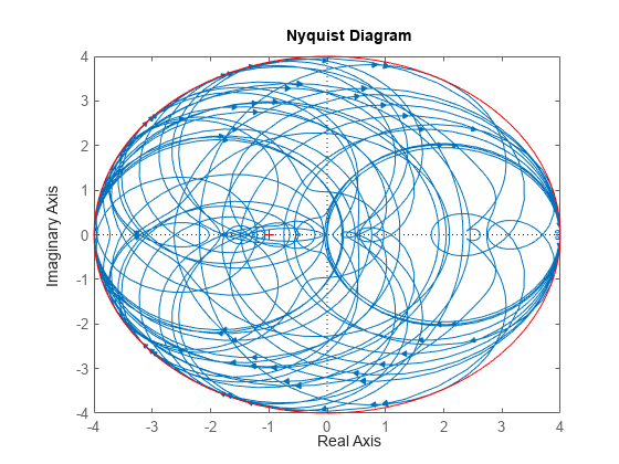
Plot the Nyquist plot of these samples and add a disk of radius 4, the gain bound of del.
nyquist(delS) hold on; theta = linspace(-pi,pi); plot(del.Bound*exp(sqrt(-1)*theta),'r'); hold off;

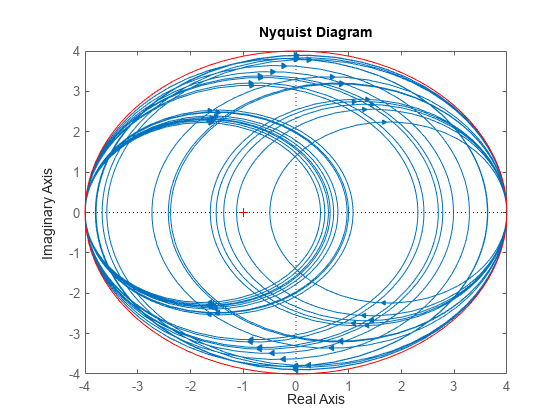
Change SampleStateDimension to 1, and repeat entire procedure. The Nyquist plots again satisfy the gain bound, but the Nyquist plots are all circles, indicative of 1st order systems.
del.SampleStateDimension = 1; delS = usample(del,30); nyquist(delS) hold on; theta = linspace(-pi,pi); plot(del.Bound*exp(sqrt(-1)*theta),'r'); hold off;

With SampleStateDimension = 1, all Nyquist plots touch the gain boundary at either (–1,0) or (1,0) (frequency = 0 or Inf). Higher sampling dimension yields a Nyquist curve that reaches the gain bound at more frequencies, yielding more thorough coverage.
Create a umargin object using the default SampleStateDimension. The umargin block models uncertain gain and phase. The modeled variations are within bounded ranges. For this example use a umargin block that captures relative gain variations of a factor of two in either direction, and phase variations of ±30°.
DGM = getDGM(2,30,'tight'); F = umargin('F')
Uncertain gain/phase "F" with relative gain change in [0.5,2] and phase change of ±36.9 degrees. Block Properties
The samples of a umargin block are also state-space models.
Fs = usample(F,30); size(Fs)
30x1 array of state-space models.
Each model has 1 outputs, 1 inputs, and 3 states.
Plot the samples on the Nyquist plane.
nyquist(Fs)

The Nyquist plot of any sample of F stays within the disk of uncertainty modeled by F. To confirm this bound, use plot to examine the uncertainty disk. Compare the Nyquist plot above with the right side of the following plot.
plot(F)

For further details about the gain and phase uncertainty model, see umargin.