Simulate Path Following on Speedgoat Real-Time Target Machine

Since R2025a

This example shows how to perform real-time simulations for path following in a complex environment using Speedgoat real-time target machines. You can use this example for testing and validation of the vehicle's ability to accurately follow paths in a complex and dynamic environment.

To run this example, you must install the Speedgoat I/O Blockset and the Simulink® Real-Time™ support package.

• To install the Speedgoat I/O Blockset, go to www.speedgoat.com/extranet, the Speedgoat Customer Portal. Follow the instructions to download and install the Speedgoat I/O Blockset.

• Download and install the Simulink Real-Time support Package using the Add-On Explorer. For more information about installing add-ons, see Get and Manage Add-Ons.

System Configuration

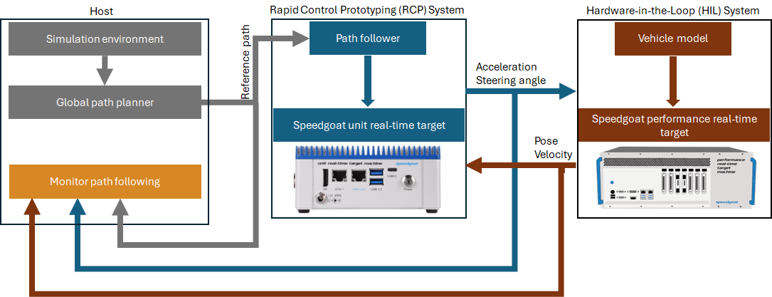
In this example, you will use three distinct systems, each configured for specific tasks within the simulation framework.

• Host - The host computer contains a Simulink model that act as the main interface to manage the overall simulation and coordinate interactions between the Rapid control prototyping (RCP) and the Hardware-in-the-Loop (HIL) system.

• Rapid Control Prototyping system - This system deploys the Simulink® model for path following on a Speedgoat performance real-time target machine to guide the target vehicle along a pre-defined path. The system computes the steering angle and acceleration values.

• Hardware-in-the-Loop system - This system deploys the Simulink® model for representing vehicle dynamics on a Speedgoat unit real-time target machine to simulate the vehicle's response. The HIL system receives the steering angles and acceleration commands as inputs from the RCP system and simulates the vehicle maneuver. The system sends feedback on the vehicle's current state, including position and velocity to the RCP system for validation and error correction. By comparing the vehicle's current state with the desired trajectory, the RCP system calculates positional and heading errors, adjusting steering and acceleration commands accordingly. This ensures the vehicle remains on course, adapting dynamically to changes in speed or direction, and effectively handling any deviations from the path for smooth and precise navigation.

The rest of the example explains the Simulink models within the simulation framework and how to deploy and run the Simulink models on the Speedgoat real-time target machines.

Simulation Framework

This section explains these three Simulink models that comprise the simulation frame work for real-time path following simulation.

1. Host Model: The model provides the input scenario and the global reference path for path following. Additionally, it includes a monitoring subsystem that allows you to visualize the simulation results. The model uses helperPlanRoadNetworkPath helper function to compute the global reference path.

2. Path Follower Model: This model implements the path following technique and computes the control inputs, specifically the acceleration and the steering angle. The Path Follower model uses the Pure Pursuit block and the PID Controller block to compute the acceleration and steering angle values.

3. Vehicle Model: This model simulates the vehicle's motion and response to the control inputs by considering the physical dynamics of the vehicle. The model uses a 3 Degrees of Freedom (3DOF) Bicycle Model, coupled with a simple driveline system.

These models use these helper functions to load the parameters required for the simulation.

• helperScenarioParams helper functions to load the simulation environment and global path planning parameters.

• helperPathFollowerParams and helperVehicleParams helper functions to load the controller and vehicle parameters, respectively.

Review Host Model

Open the Simulink model that runs on host computer and provides the input scenario and the global reference path for path following.

open_system("Host")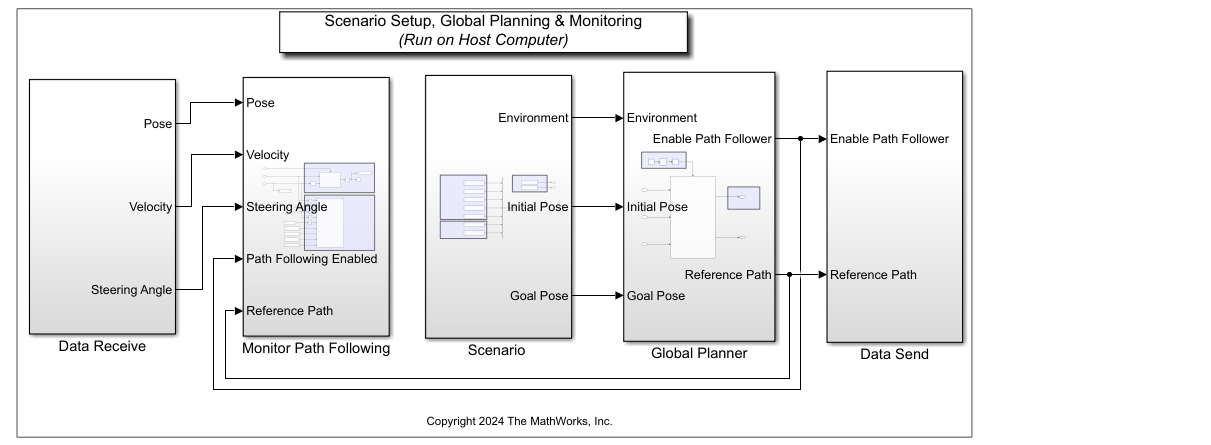

The model is composed of three key subsystems: Scenario, Global Planner, and Monitor Path Following. The Data Send block transmits data to the RCP system. The Data Receive block receives data from both the RCP and HIL systems. The Data Send and Data Receive blocks uses the User Datagram Protocol (UDP) for communication.

Scenario Subsystem

The Scenario subsystem sets up the input scenario for path following using the helperScenarioParams helper function. The scenario and the scenario parameters are stored to a .mat file. This function loads these parameters:

• Road network information - Nodes, edges, and edge costs that define the structure and traversal costs of the road network.

• Cached paths - Precomputed paths for efficient path finding, along with a mapping from edges to these paths.

• Reference path size - A fixed size for the path to ensure consistency in path planning outputs. Increasing the reference path size can result in a more detailed path with additional waypoints, which may lead to smoother navigation and more precise path following. However, it also increases the computational load. In this example, the reference path size is set to 500.

• Sampling time - The interval at which the simulation updates. In this example, the sampling time is set to 0.001 seconds.

• Initial and goal poses - The starting and ending positions and orientations for the vehicle within the simulation.

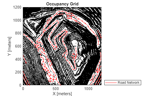
You can specify custom values for the input scenario and scenario parameters by using the helperScenarioParams function. First, store the scenario and scenario parameters in a .mat file. Then, use the helperScenarioParams function to load the input scenario and scenario parameters for simulation. This example uses an open pit mine environment as the input scenario. The scenario and the scenario parameters are stored in the OpenPitMineRoadNetwork.mat file.

Load the input scenario and the corresponding nodes and cached paths into the MATLAB® workspace.

T = load("OpenPitMineRoadNetwork.mat","mapMatrix","nodes","cachedPaths");

Create an occupancy map of the input scenario.

map = occupancyMap(T.mapMatrix);

Visualize the map and the road network path.

figure
show(map)
hold on
scatter(T.nodes(:,1),T.nodes(:,2),5,"o","r")
pathIds = unique(T.cachedPaths(:,1)) ;
for i=1:length(pathIds)
    id = find(pathIds(i)==T.cachedPaths(:,1));
    h = plot(T.cachedPaths(id,2),T.cachedPaths(id,3),"r");
end
legend(h,"Road Network",Location="southeastoutside")

Global Planner Subsystem

The Global Planner subsystem uses the helperPlanRoadNetworkPath helper function to compute the global reference path by taking into account the scenario parameters and the vehicle's minimum turning radius. The planner computes the optimal path by using:

1. A* algorithm to determine the best route through the road network graph, from the start node to the goal node, utilizing cached paths for efficiency.

2. For the entry and exit segments, the planner employs Hybrid A* to generate precise paths, ensuring the vehicle moves forward during these maneuvers.

3. Finally, it merges the entry, road network, and exit paths into a single continuous path. The combined path is then adjusted to match the specified reference path size, ensuring uniform spacing between waypoints.

Once the global reference path is computed, the global planner activates the RCP system to initiate path following.

Monitor Path Following Subsystem

The Monitor Path Following subsystem monitors whether the vehicle has reached the goal point, evaluates the tracking error in real-time, and generates visual outputs. The subsystem uses a MATLAB® Function block for monitoring the path following results. This block implements a custom MATLAB code to generate visual outputs, facilitate the assessment of the vehicle's path-following performance directly within the Simulink model. When the vehicle reaches its designated goal point, the subsystem automatically stops the simulation. The subsystem displays these results in real-time.

• Vehicle path - This refers to the visualization of the vehicle's actual path compared to the desired path. It shows how accurately the vehicle is able to follow the reference path.

• Linear velocity - This graph displays the changes in the vehicle's speed as it moves along the path. You can use this plot to analyze acceleration and deceleration patterns and determine if the vehicle maintains the desired velocity throughout its maneuver.

• Steering angle - This plot shows how the steering angle changes over time as the vehicle navigates the path. It provides insights into the control inputs required to maintain the desired path and can highlight any excessive steering adjustments.

• Tracking error - This graph illustrates the deviation of the vehicle from the desired path, measured as the Euclidean distance between the vehicle's current position and the nearest point on the reference path.

Review Path Follower Model

Load and open the Simulink model for path following.

open_system("PathFollower")

The Simulink model for path following contains three subsystems: Data Receive, Path Follower, and Data Send.

Data Receive and Data Send Subsystems

The Data Receive subsystem collects data from the host Simulink model and the HIL system. It sends this data to the Path Follower subsystem. The host model provides the reference path and a trigger signal to enable the Path Follower after computing the global reference path. The HIL system supplies the vehicle's current pose and velocity to the Path Follower subsystem. These inputs help correct errors and calculate the steering angle and acceleration commands to maneuver the vehicle along the reference path at a desired velocity.

The Data Send subsystem transmits the steering and acceleration commands to the HIL system to control the vehicle's maneuver and to the host Simulink model for visualization purposes.

Path Follower Subsystem

The Path Follower subsystem computes the acceleration and steering angle for path following. The subsystem uses the helperPathFollowerParams and the helperVehicleParams helper functions to specify the controller and vehicle parameters, respectively, for computing the acceleration and steering angle.

The helperPathFollowerParams function loads these parameters:

• Desired Linear Velocity - Starting speed that a vehicle aims to reach or maintain at the beginning of a maneuver.

• Lookahead distance - Distance ahead of the vehicle's current position that the path follower considers to determine the desired trajectory. A larger lookahead distance can lead to smoother path following and improved stability but may result in slower response times. Conversely, a smaller lookahead distance allows for faster response but can cause higher oscillations and potential instabilities, especially during tight maneuvers. In this example, this parameter value is set to 3m.

• P gain of PID controller - Proportional gain (P gain) determines the strength of the controller's immediate response to an error. A higher P gain increases the system's responsiveness to changes and performs quicker adjustments to minimize the error. However, if set too high, it can lead to overshooting and oscillations. Conversely, a lower P gain results in a less responsive system, which may reduce overshooting but can also lead to slower error correction and potentially a steady-state error. In this example, the P gain for the longitudinal and the steering controller is empirically set to 10.

• I gain of PID controller - Integral gain (I gain) determines the controller's ability to eliminate steady-state errors by integrating the accumulated error over time. A higher I gain reduces steady-state errors but can cause overshoot and oscillations, potentially leading to instability. Conversely, a lower I gain minimizes overshoot and oscillations but may result in larger steady-state errors. In the example, the I gain for the longitudinal and steering controller is empirically set to 0.1.

The helperVehicleParams helper function loads these vehicle parameters, in addition to other vehicle dynamics parameters:

• Maximum lateral acceleration - Highest lateral acceleration the vehicle can handle safely during turn.

• Maximum acceleration - Maximum rate at which the vehicle can increase its speed.

• Maximum deceleration - Highest rate at which the vehicle can safely decrease its speed.

• Maximum steering angle rate - Maximum speed at which the steering angle can change.

Open the Path Follower subsystem.

open_system("PathFollower/Path Follower")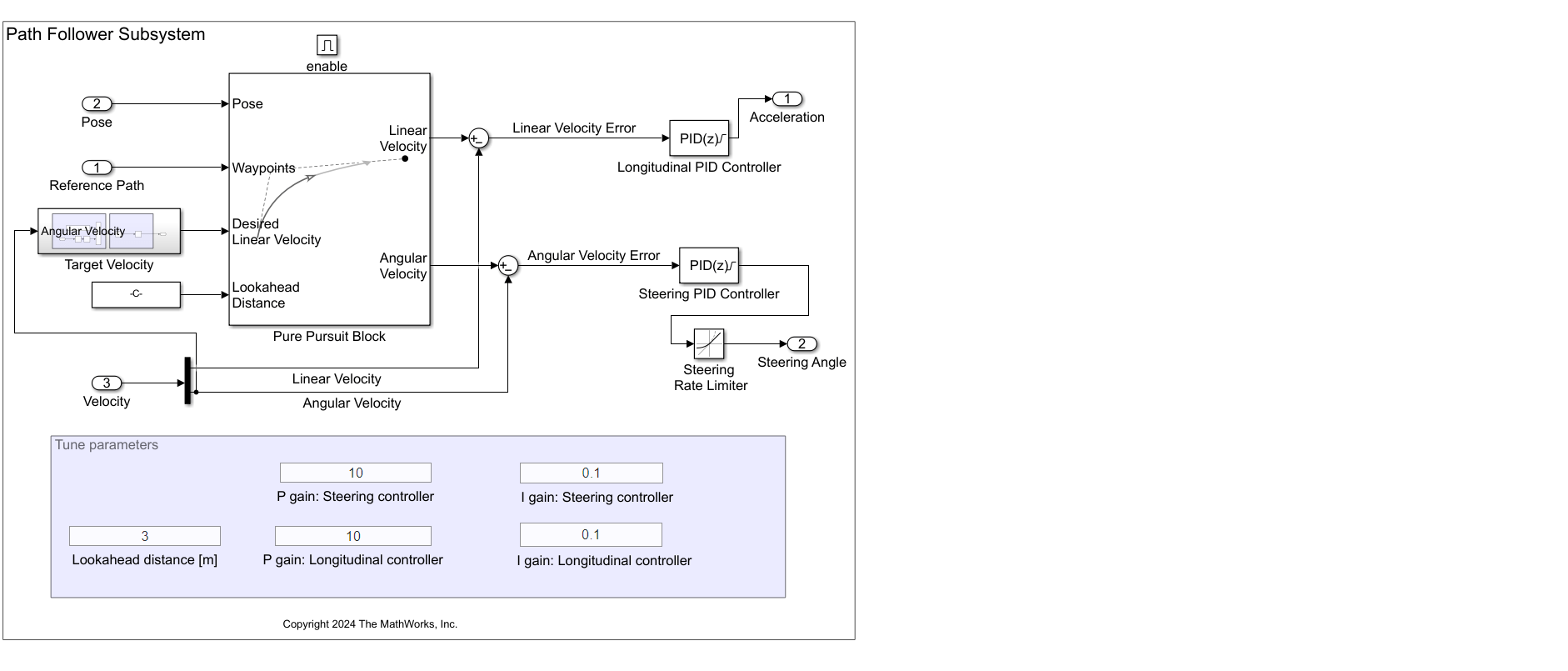

The Path Follower subsystem computes the acceleration and steering angle using these three main components:

• MATLAB Function Block - Computes the target linear velocity using the vehicle's maximum lateral acceleration and the current angular velocity from the HIL system. The block ensures that the target linear velocity does not exceed the desired linear velocity. In this example, the desired velocity is set to 10 m/s. The block also ensures that any changes in speed occur within the maximum acceleration and deceleration limits. This prevents sudden or abrupt changes in speed, maintaining a smooth velocity profile.

• Pure Pursuit Block - Computes the final linear velocity and angular velocity using the lookahead distance, reference path, target linear velocity, and the current pose of the vehicle.

• Longitudinal PID Controller - Computes acceleration based on the error between the current linear velocity returned by the HIL system and the linear velocity computed using the Pure Pursuit block.

• Steering PID Controller - Computes steering angle based on the error between the current angular velocity returned by the HIL system and the angular velocity computed using the Pure Pursuit block.

You can tune the controller parameters by using the edit box in the Path Follower subsystem. Alternately, you can also edit the helperPathFollowerParams helper function to specify custom values for the controller parameters.

Review Vehicle Model

Open the Vehicle model.

load_system("Vehicle")
open_system("Vehicle/Vehicle")

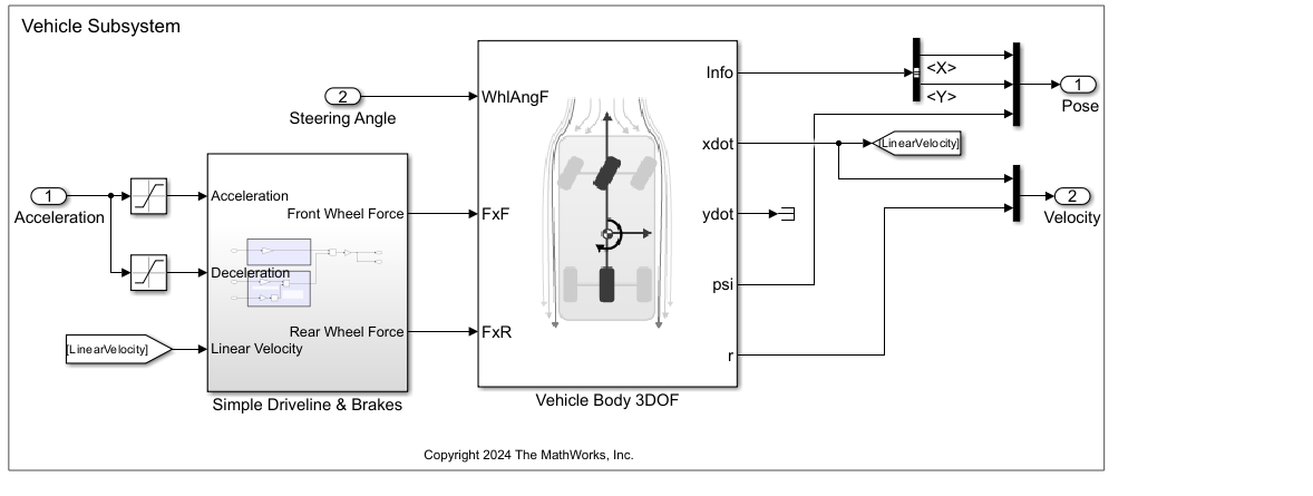
The vehicle model uses the Vehicle Body 3DOF block to calculate longitudinal, lateral, and yaw motions. The Vehicle Body 3DOF block considers the body mass and aerodynamic drag acting between the axles due to acceleration and steering. The computed final pose and velocity specify the vehicle's updated state in the simulation environment.

The helperVehicleParams helper function specifies the longitudinal and lateral vehicle parameters that the Vehicle Body 3DOF block requires to compute the vehicle's final pose and velocity. For information on the longitudinal and lateral vehicle parameters, see Longitudinal and Lateral parameters in . The vehicle model preloads the helperVehicleParameters function, enabling the Vehicle Body 3DOF block to automatically access the necessary parameter values.

Configure UDP Send and Receive Blocks

Configure the UDP Send and UDP Receive blocks in the Simulink models with valid IP addresses. The helperIPAddresses helper function specifies the IP addresses for the Host, Path Follower, and the Vehicle models. You must edit the helper function to specify custom values for the IP addresses.

% Rapid Control Prototyping (RCP) system for Path Follower Model
ipAddress.rcpSystem = '127.0.0.1';
% Hardware-in-the-Loop (HIL) System for the Vehicle Model
ipAddress.hilSystem = '127.0.0.2';
% Host computer
ipAddress.hostSystem = '120.0.0.1';

Deploy Simulink Models on Speedgoat

This section explains how to deploy the Path Follower and Vehicle Simulink models on the Speedgoat real-time target machines to implement the RCP and HIL systems, respectively. To deploy the Simulink models on Speedgoat real-time target machines by using the graphical user interface (GUI) or an programmatic approach.

GUI Approach

To deploy the models on the target machines using GUI, follow step 1 to step 4:

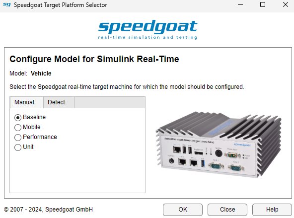
Step 1: In Simulink Editor, from the Apps tab, click Simulink Real-Time. Select the appropriate Speedgoat target platform.

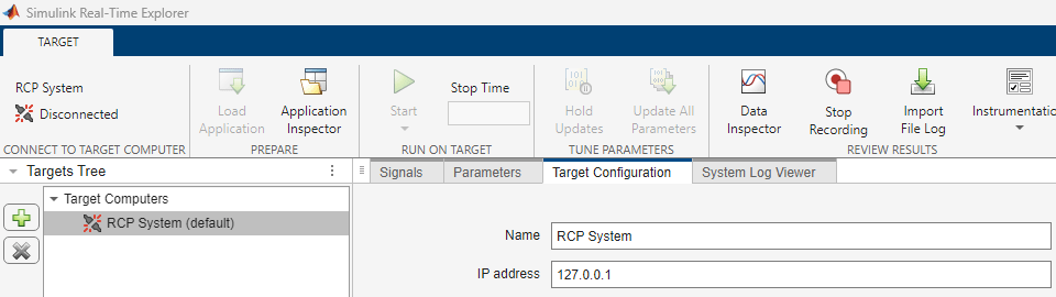
When you open the app, a Real-Time tab is added to the toolstrip. In the Real-Time tab, from the targets list, click SLRT Explorer.

Step 2: Configure RCP and HIL Systems

Specify the target computer name as RCP System and the IP address of the Path Follower model. Toggle the Disconnected indicator to Connected to connect to the target computer.

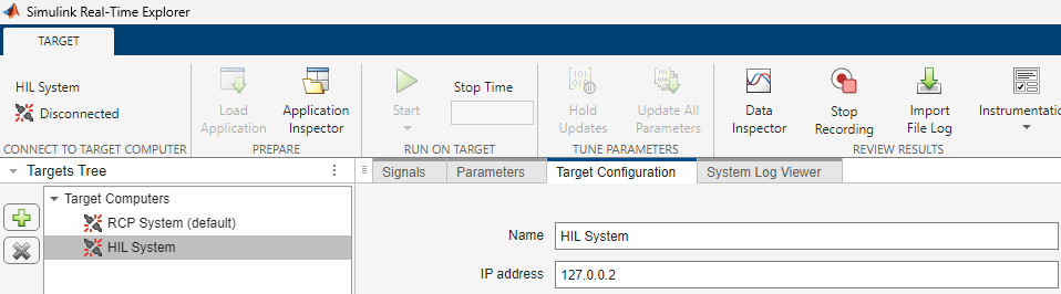
In the Targets pane, click Add target to add a target computer for HIL system. Specify the target computer name as HIL System and the IP address of the Vehicle model. Toggle the Disconnected indicator to Connected to connect to the target computer.

Step 3: Deploy Path Follower Model on RCP System

Open the Path Follower model. In the Real-Time tab, select RCP System. Ensure that the RCP system is connected to the Speedgoat target machine. Select Run on Target to compile and deploy the Path Follower model on the RCP system.

open_system("PathFollower")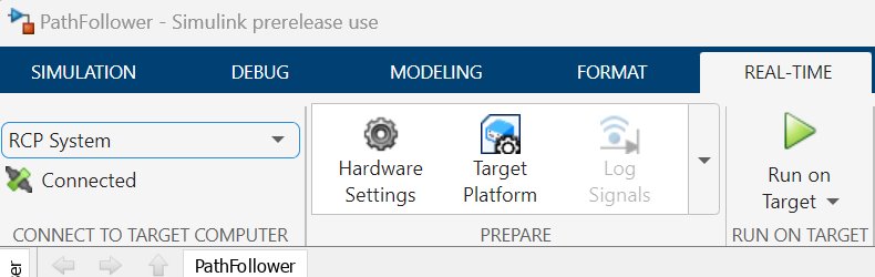

Step 4: Deploy Vehicle Model on HIL System

Open the Vehicle model. In the Real-Time tab, select HIL System. Ensure that the HIL system is connected to the Speedgoat target machine. Select Run on Target to compile and deploy the Vehicle model on the HIL system.

open_system("Vehicle")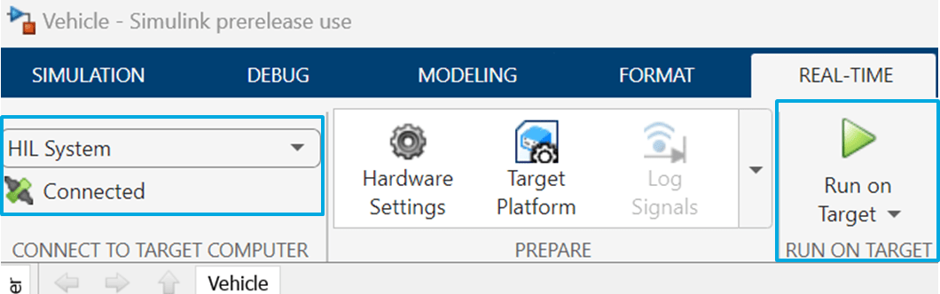

Programmatic Approach

Alternately, you can use the programmatic approach to configure and deploy the RCP and HIL systems. Use the helperRealTimeSimulation helper function to specify the Simulink model names to deploy the models on the target machines. The helperRealTimeSimulation helper function fetches the IP addresses using the helperIPAddresses helper function.

model = "PathFollower";
helperRealTimeSimulation(model)
model = "Vehicle";
helperRealTimeSimulation(model)

Run Simulation and Visualize Results

Open the Host model and run the simulation from the SIMULATION tab.

open_system("Host")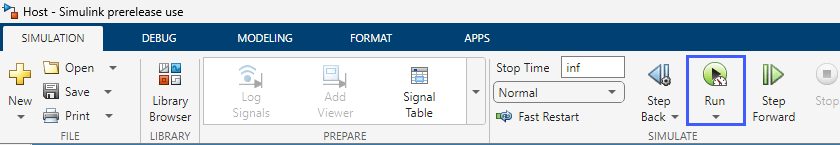

The Monitor Path Following subsystem in the Host Model displays the real-time simulation results.

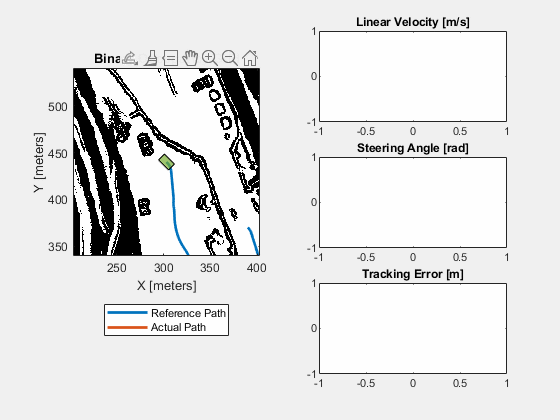
• You can notice that the actual vehicle path is much closer to the reference path. Smaller deviations between these paths indicate the system's accuracy. In areas with high curvature, there may be higher deviations between the actual vehicle path and the reference path. To reduce these deviations and enhance overall performance, you can adjust the controller parameters.

• The linear velocity plot shows how the vehicle's velocity varies over time. The controller attempts to maintain a desired velocity of 10 m/s on straighter portions of the road. However, to ensure vehicle stability, it slows down on high curvature portions of the road.

• The steering angle plot illustrates how the control commands for the steering angle are adjusted along the path. The steering angle generally follows the curvature of the input reference path, with higher curvature in the input path leading to larger steering angles.

• The tracking error plot quantifies the quality of path following by measuring the shortest distance between the actual vehicle path and the reference path. The lower this value, the better the performance. You can observe that the tracking error reaches 4 meters at two locations, which correspond to the high curvature portions of the path. To minimize this error, you can try tuning the controller parameters or use advanced path followers like TEB (Timed Elastic Band) or MPPI (Model Predictive Path Integral).

Check task execution time

For maintaining the stability and reliability of the real-time system, the maximum execution time for the real-time target machines must be less than the base rate. You can use the TET Monitor to view the task execution time for the real-time application running on the Speedgoat® target machines. From the Simulink Editor, in the Real-Time tab, select TET Monitor to view the task execution time.

Stop application

Use the Stop Application button on the RUN ON TARGET tab to stop the real-time applications running on the Speedgoat target machines.