Constrain Links of Excavator for Earth Moving

Since R2026a

Earth-moving tasks like digging and grading impose constraints on how you can position the stick and boom of an excavator arm. This example shows how to use generalized inverse kinematics (GIK) to find excavator arm joint angles that satisfy these constraints. Then the example shows how to create continuous trajectories between these arm joint angles, either by interpolating between joint angles or by applying resolved-rate motion control with the geometric Jacobian.

If you already have excavator joint angles and you want to learn more about motion planning using those joint angles, see the Plan Collision-Free Path for Excavator Arm in MATLAB With Lidar Data example.

Load Excavator Model

Load the rigid body tree model of an excavator, and specify the names of the stick and bucket bodies in the rigid body tree model.

load("MathScavator9000.mat","excavatorRBT")
stickBody = "boom_stick_link";
bucketBody = "stick_bucket_link";

Add a frame, "bucket_tooth", at the middle tooth of the bucket.

bucketToothFrame = "bucket_tooth";
addFrame(getBody(excavatorRBT,bucketBody), ...
    bucketToothFrame,bucketBody, ...
    trvec2tform([0 -1.8 0])*trvec2tform([0 0 1]));

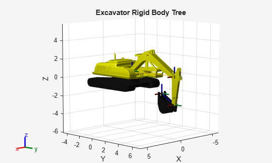
Show the excavator, increasing the frame size to make the frames more visible.

figure
show(excavatorRBT,FrameSize=1);
title("Excavator Rigid Body Tree")
axis auto

Dig at Desired Depth and Attack Angle

To perform digging tasks, the excavator bucket must reach the correct height with the correct orientation. These two parameters are called the digging depth and attack angle, respectively.

• Digging Depth — This is the vertical z-axis distance between the excavator base frame and the point where the origin of the bucket tooth frame must enter the ground.

• Attack Angle — The angle between the z-axis of the bucket tooth frame and the tangent line to the digging arc at the bucket tip. The attack angle determines how the bucket enters the ground, and is measured at the point where the origin of the bucket tooth frame follows a circular arc centered at the boom-stick joint.

This figure shows these parameters:

Define the digging depth and attack angle.

depth = 5; % meters
attackAngle = deg2rad(12);

To specify the digging depth and attack angle constraints to a GIK solver, you must define a constraintCartesianBounds object and a constraintOrientationTarget object, respectively.

Define a Cartesian bounds constraint that places the bucket body at 0 meters in the x-direction, at least 2 meters in the y-direction, and at a minimum digging depth.

diggingDepthConstraint=constraintCartesianBounds(bucketToothFrame, ...
	Bounds=[0 0; 4 inf; -inf -depth]);

Define an orientation constraint to satisfy the desired attack angle.

attackAngleConstraint = constraintOrientationTarget(bucketToothFrame, ...
	ReferenceBody=stickBody, ...
	TargetOrientation=eul2quat([0 0 pi/2+attackAngle]));

Create a generalizedInverseKinematics solver to find joint angles that satisfy the geometric constraints. Use the home joint angles of the excavator rigid body tree as the initial guess for the solver.

initialJointAngGuess = homeConfiguration(excavatorRBT);
gik = generalizedInverseKinematics(RigidBodyTree=excavatorRBT, ...
	ConstraintInputs={'cartesian','orientation'});

Solve for the excavator joint angles.

[digAttackJntAng,solInfoDigAttackAng] = gik(initialJointAngGuess, ...
	diggingDepthConstraint,attackAngleConstraint)

digAttackJntAng = 1×4

         0   -0.1638   -0.1192   -1.7802

solInfoDigAttackAng = struct with fields:
              Iterations: 21
       NumRandomRestarts: 0
    ConstraintViolations: [1×2 struct]
                ExitFlag: 1
                  Status: 'success'

assert(strcmp(solInfoDigAttackAng.Status,"success"))

Visualize the excavator with the joint angles that satisfy the desired digging depth and attack angle.

show(excavatorRBT,digAttackJntAng,FrameSize=0.5);
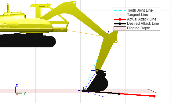
hold on

Use helper functions to show the digging depth and attack lines.

digDepthPlane = exampleHelperCreatePlaneAtZ(-depth);
[toothLine,tangent,actAttkLine,desAttkLine] = ...
    exampleHelperPlotAttackAngle(excavatorRBT,digAttackJntAng,attackAngle);

legend([toothLine tangent actAttkLine desAttkLine digDepthPlane],...
    {'Tooth Joint Line','Tangent Line','Actual Attack Line', ...
    'Desired Attack Line','Digging Depth'})
title("Minimum Depth And Desired Attack Angle")
hold off

% Set viewing properties to focus on the bucket and stick
view([90 0])
camva(2.2)
zlim([-13 10])
ylim([-9 13])

Dig at Desired Depth with Vertical Stick

In the previous GIK solution, the stick link is not vertical because the solver orients it to achieve an attack angle. If the task requires the stick to be vertical while digging to a certain depth, you can achieve this by imposing an orientation constraint on the stick. This figure shows the stick in the vertical position.

You can find the orientation of the stick for any set of joint angles using the getTransform object function. This function returns the homogeneous transformation matrix, containing position and orientation, of the stick body with respect to the base of the excavator. To demonstrate this, calculate the stick orientation for the previous solution and convert the transformation matrix to Euler angles.

stickPose = getTransform(excavatorRBT,digAttackJntAng,stickBody);
stickEul = tform2eul(stickPose)

stickEul = 1×3

         0         0   -0.2829

Specify a target-orientation constraint for the stick body such that it is vertical. By default, the target orientation is an identity rotation, which means that the frame of the stick must be oriented in the same way as the base frame of the excavator.

stickVerticalConstraint = constraintOrientationTarget(stickBody);
[digVertStickJntAng,solinfoDigVertStick] = gik(initialJointAngGuess, ...
    diggingDepthConstraint,stickVerticalConstraint);
disp(solinfoDigVertStick)

              Iterations: 37
       NumRandomRestarts: 0
    ConstraintViolations: [1×2 struct]
                ExitFlag: 1
                  Status: 'success'

assert(strcmp(solinfoDigVertStick.Status,"success"))

Verify the orientation for the constrained joint angles.

constrainedStickEul = tform2eul(getTransform(excavatorRBT,digVertStickJntAng,stickBody))

constrainedStickEul = 1×3
10-8 ×

         0         0   -0.2606

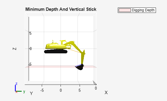
figure
show(excavatorRBT,digVertStickJntAng);
title("Minimum Depth And Vertical Stick")
hold on
digDepthPlane = exampleHelperCreatePlaneAtZ(-depth);
legend(digDepthPlane,"Digging Depth")
view(90,0)
hold off

Unload Bucket After Digging

To unload the bucket after digging, the bucket must be at the correct position, typically above a dump truck bed.

Define a target-position constraint that places the bucket at an unloading position. In this example, place it at position tgtpos in the coordinate system of the excavator base.

tgtpos = [-2.4 6 5];
positionBucketLinkConstraint = constraintPositionTarget(bucketBody,TargetPosition=tgtpos);
gik = generalizedInverseKinematics(RigidBodyTree=excavatorRBT,ConstraintInputs={'position'});
unloadingJntAng = gik(homeConfiguration(excavatorRBT),positionBucketLinkConstraint);
figure
show(excavatorRBT,unloadingJntAng);
title("Unloading Position")
view(90,0);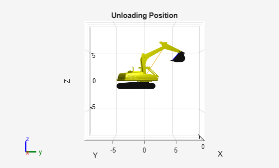

Move Between Constrained Joint Angles

To move smoothly between the constrained excavator joint angles, such as digging and unloading, fit a quintic polynomial trajectory between the joint angles. This approach generates a smooth joint trajectory, but it does not account for potential collisions with the environment. For collision-aware planning, use a motion planner such as manipulatorRRT.

Specify time points, and set the joint-angle waypoints to the position for digging with an attack angle, then to the position for digging with a vertical stick position, and finally to the unloading position. Add a joint angle waypoint that rotates the bucket to unload it.

tpts = [0 3 10 12];
wpts = [digAttackJntAng;
	digVertStickJntAng;
	unloadingJntAng;
	[unloadingJntAng(1:end-1) -pi/2]]';

Specify the query time vector with 0.05 second spacing between the beginning and ending time points.

tvec = tpts(1):0.05:tpts(end);
digJntAngTraj = quinticpolytraj(wpts,tpts,tvec);

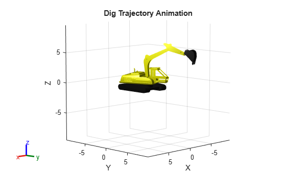
For every interpolation of joint angles in the trajectory, visualize the rigid body tree of the excavator.

rc = rateControl(100);
figure;
ax = show(excavatorRBT,digJntAngTraj(:,1)',Frames="off",DisplayBodyDetails="off");
title("Dig Trajectory Animation")
hold on
for i = 1:size(digJntAngTraj,2)
	show(excavatorRBT,digJntAngTraj(:,i)',Parent=ax,FastUpdate=true,PreservePlot=false,Frames="off",DisplayBodyDetails="off");
	drawnow
    waitfor(rc);
end
hold off

Grading Trajectory

While this example has focused on moving between discrete poses, some tasks, such as grading, require the excavator to follow a continuous path at a specified velocity and orientation. For these tasks, you can use velocity-based control rather than interpolating between joint angles.

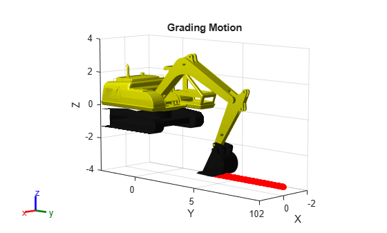
To perform a grading motion, move the bucket in the negative y-direction of the excavator base body frame. Start with a reach of 10 meters away from the excavator at the position [0 10 -3.5], digging at a depth of 3.5 meters with a linear velocity of 0.03 meters per second and a slight angular velocity of 7.5e-3 rad/s in the x-direction.

Specify the reach and digging depth using a Cartesian bounds constraint.

diggingDepthConstraint.Bounds(2,:) = [10 10];
diggingDepthConstraint.Bounds(3,:) = [-inf -3.5];

Solve for the initial set of joint angles.

gik = generalizedInverseKinematics(RigidBodyTree=excavatorRBT,ConstraintInputs={'cartesian'});
[gradeInitJntAng,solinfoGradeInit] = gik(homeConfiguration(excavatorRBT),diggingDepthConstraint)

gradeInitJntAng = 1×4

         0   -0.1396    0.9349   -2.2685

solinfoGradeInit = struct with fields:
              Iterations: 23
       NumRandomRestarts: 0
    ConstraintViolations: [1×1 struct]
                ExitFlag: 1
                  Status: 'success'

ax = show(excavatorRBT,gradeInitJntAng,Frames="off",DisplayBodyDetails="off");
title("Grading Motion")
zlim([-4 4])
ylim([-3 10])
xlim([-2 2])
hold on

Specify the linear velocities.

vx = 0;
vy = -0.03;
vz = 0;
dv = [vx,vy,vz].';

Specify the angular velocities.

wx = -7.5e-3;
wy = 0;
wz = 0;
dw = [wx,wy,wz].';
dt = 1;

Use the manipulator Jacobian to compute the joint velocities from the desired bucket-tooth-frame velocities. Then, update the current joint angles based on this joint velocity. This resolved-rate motion control approach achieves accuracy comparable to solving inverse kinematics at every step, but is more computationally efficient [1].

for tstep = 0:dt:200
    % Compute the geometric Jacobian at the current joint angles
    J = geometricJacobian(excavatorRBT,gradeInitJntAng,bucketToothFrame);

    % Calculate joint velocities required to achieve the desired end-effector velocities
    dq = (pinv(J)*[dw; dv]).';

    % Get bucket tooth position for visualizing grading path
    prevtoothpos = tform2trvec(getTransform(excavatorRBT,gradeInitJntAng,bucketToothFrame));

    % Update the joint angles using the calculated joint velocities
    gradeInitJntAng = gradeInitJntAng+dq*dt;

    % Get the new position of the bucket tooth after the joint angle update
    currtoothpos = tform2trvec(getTransform(excavatorRBT,gradeInitJntAng,bucketToothFrame));

    % Visualize the excavator with the current joint angles
    show(excavatorRBT,gradeInitJntAng,Parent=ax,FastUpdate=true,PreservePlot=false,Frames="off",DisplayBodyDetails="off");

    % Plot trajectory of bucket teeth
    plot3([prevtoothpos(1) currtoothpos(1)], ...
        [prevtoothpos(2) currtoothpos(2)], ...
        [prevtoothpos(3) currtoothpos(3)],"r.",MarkerSize=20)
    drawnow
    waitfor(rc);
end
hold off

References

[1] Haviland, Jesse, and Peter Corke. “Manipulator Differential Kinematics: Part I: Kinematics, Velocity, and Applications [Tutorial].” IEEE Robotics & Automation Magazine 31, no. 4 (2024): 149–58. https://doi.org/10.1109/MRA.2023.3270228.

Copyright 2025 The MathWorks, Inc.,