Richards-Kuroda Workflow for RF Filter Circuit
This example shows how to apply Richards-Kuroda workflow to an RF filter circuit.
Create a lowpass LC-Pi Chebyshev filter with the passband frequency of 1 GHz, passband attenuation of 0.5 dB, and filter order of 5.
Fp = 1e9;
Ap = 0.5;
Ord = 5;
r = rffilter(FilterType="Chebyshev",ResponseType="Lowpass",Implementation="LC Pi",PassbandFrequency= ...
    Fp,PassbandAttenuation=Ap,FilterOrder=Ord);
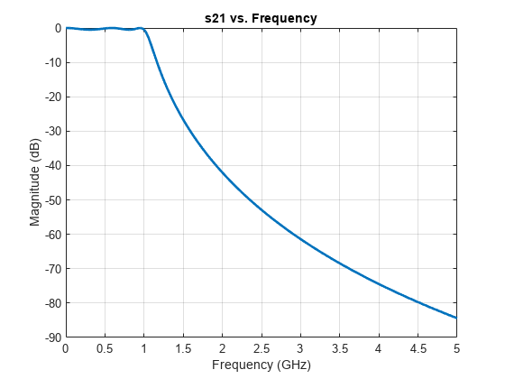
Plot the S21 parameter of the RF filter.
frequencies = linspace(0,5*Fp,1001);
rfplot(r, frequencies)
Convert the lumped-element filter to a distributed-element-based circuit at the operating frequency of 1 GHz using the richards function.
txCkt = richards(r,1e9)
txCkt =
  circuit: Circuit element

    ElementNames: {'C_tx'  'L_tx'  'C_1_tx'  'L_1_tx'  'C_2_tx'}
        Elements: [1×5 txlineElectricalLength]
           Nodes: [0 1 2 3 4 5 6]
            Name: 'unnamed'
Show the circuit properties in a table using the tableCircuitProperties function. You can find the source code for this helper function in the Supporting Functions section at the end of this example.
tableCircuitProperties(txCkt,'Name','StubMode','Termination','Z0')
       Name        StubMode     Termination      Z0
    __________    __________    ___________    ______

    {'C_tx'  }    {'Shunt' }     {'Open' }     29.312
    {'L_tx'  }    {'Series'}     {'Short'}     61.481
    {'C_1_tx'}    {'Shunt' }     {'Open' }     19.679
    {'L_1_tx'}    {'Series'}     {'Short'}     61.481
    {'C_2_tx'}    {'Shunt' }     {'Open' }     29.312
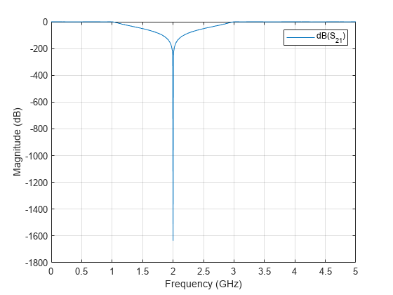
Plot the S21 parameter of distributed-element-based filter circuit. The RF plot shows that distributed and lumped filter behavior overlap close to the operating frequency and diverge significantly at higher frequencies. This occurs due to the frequency-periodic nature of distributed elements.
rfplot(sparameters(txCkt, frequencies),2,1)

The distributed-element-based circuit in txCkt circuit is not practical since all stubs essentially stem from the same point in space. To separate the stubs and use only shunt stubs that are easier to implement as microstrip lines, insert unit elements in a sequence and apply Kuroda's identities.
Add unit elements at the edges of the txCkt, operating at 1 GHz with the characteristic impedance of 50 ohms. The edges of the circuit are port 1 of the first circuit element C_tx and port 2 of the last circuit element C_2_tx.
 txCkt_UE = insertUnitElement(txCkt,'C_tx',1,1e9,50);
 txCkt_UE = insertUnitElement(txCkt_UE,'C_2_tx',2,1e9,50)
txCkt_UE =
  circuit: Circuit element

    ElementNames: {'C_tx_p1_elem_UE'  'C_tx'  'L_tx'  'C_1_tx'  'L_1_tx'  'C_2_tx'  'C_2_tx_p2_elem_UE'}
        Elements: [1×7 txlineElectricalLength]
           Nodes: [0 1 2 3 4 5 6 7 8]
            Name: 'unnamed'
Show the circuit properties in a table.
tableCircuitProperties(txCkt_UE,'Name','StubMode','Termination','Z0')
            Name               StubMode         Termination         Z0
    _____________________    ____________    _________________    ______

    {'C_tx_p1_elem_UE'  }    {'NotAStub'}    {'NotApplicable'}        50
    {'C_tx'             }    {'Shunt'   }    {'Open'         }    29.312
    {'L_tx'             }    {'Series'  }    {'Short'        }    61.481
    {'C_1_tx'           }    {'Shunt'   }    {'Open'         }    19.679
    {'L_1_tx'           }    {'Series'  }    {'Short'        }    61.481
    {'C_2_tx'           }    {'Shunt'   }    {'Open'         }    29.312
    {'C_2_tx_p2_elem_UE'}    {'NotAStub'}    {'NotApplicable'}        50
Plot the S21 parameter of the new circuit txCkt_UE. The RF plot shows that the addition of unit elements does not change the power magnitude behavior of the circuit, and thus this RF plot shows the same characteristics of the S21 parameter as the distributed-element-based filter circuit.
rfplot(sparameters(txCkt_UE, frequencies),2,1)

Apply Kuroda's identities to the first two and last two elements of the circuit. For more information, see Kuroda's Transformation.
txCkt_Kur = kuroda(txCkt_UE,'C_tx_p1_elem_UE','C_tx');
txCkt_Kur = kuroda(txCkt_Kur,'C_2_tx','C_2_tx_p2_elem_UE')
txCkt_Kur =
  circuit: Circuit element

    ElementNames: {'Kuroda2_R2L_of_C_tx_p1_elem_UE'  'Kuroda2_R2L_of_C_tx'  'L_tx'  'C_1_tx'  'L_1_tx'  'Kuroda1_L2R_of_C_2_tx'  'Kuroda1_L2R_of_C_2_tx_p2_elem_UE'}
        Elements: [1×7 txlineElectricalLength]
           Nodes: [0 1 2 3 4 5 6 7 8]
            Name: 'unnamed'
Show the circuit properties in a table.
tableCircuitProperties(txCkt_Kur,'Name','StubMode','Termination','Z0')
                    Name                      StubMode         Termination         Z0
    ____________________________________    ____________    _________________    ______

    {'Kuroda2_R2L_of_C_tx_p1_elem_UE'  }    {'Series'  }    {'Short'        }    31.521
    {'Kuroda2_R2L_of_C_tx'             }    {'NotAStub'}    {'NotApplicable'}    18.479
    {'L_tx'                            }    {'Series'  }    {'Short'        }    61.481
    {'C_1_tx'                          }    {'Shunt'   }    {'Open'         }    19.679
    {'L_1_tx'                          }    {'Series'  }    {'Short'        }    61.481
    {'Kuroda1_L2R_of_C_2_tx'           }    {'NotAStub'}    {'NotApplicable'}    18.479
    {'Kuroda1_L2R_of_C_2_tx_p2_elem_UE'}    {'Series'  }    {'Short'        }    31.521
Plot the S21 parameter of txCkt_Kur. The RF plot shows that, as expected, applying Kuroda's identities does not change the behavior of the circuit (as opposed to adding a unit element, applying Kuroda's identities retains both magnitude and phase behavior of the circuit).
rfplot(sparameters(txCkt_Kur, frequencies),2,1)

Add a unit elements at the edges of this circuit operating at 1 GHz with the characteristic impedance of 50 ohms.
txCkt_UE2 = insertUnitElement(txCkt_Kur,'Kuroda2_R2L_of_C_tx_p1_elem_UE',1,1e9,50);
txCkt_UE2 = insertUnitElement(txCkt_UE2,'Kuroda1_L2R_of_C_2_tx_p2_elem_UE',2,1e9,50)
txCkt_UE2 =
  circuit: Circuit element

    ElementNames: {1×9 cell}
        Elements: [1×9 txlineElectricalLength]
           Nodes: [0 1 2 3 4 5 6 7 8 9 10]
            Name: 'unnamed'
Show the circuit properties in a table.
tableCircuitProperties(txCkt_UE2,'Name','StubMode','Termination','Z0')
                         Name                            StubMode         Termination         Z0
    _______________________________________________    ____________    _________________    ______

    {'Kuroda2_R2L_of_C_tx_p1_elem_UE_p1_elem_UE'  }    {'NotAStub'}    {'NotApplicable'}        50
    {'Kuroda2_R2L_of_C_tx_p1_elem_UE'             }    {'Series'  }    {'Short'        }    31.521
    {'Kuroda2_R2L_of_C_tx'                        }    {'NotAStub'}    {'NotApplicable'}    18.479
    {'L_tx'                                       }    {'Series'  }    {'Short'        }    61.481
    {'C_1_tx'                                     }    {'Shunt'   }    {'Open'         }    19.679
    {'L_1_tx'                                     }    {'Series'  }    {'Short'        }    61.481
    {'Kuroda1_L2R_of_C_2_tx'                      }    {'NotAStub'}    {'NotApplicable'}    18.479
    {'Kuroda1_L2R_of_C_2_tx_p2_elem_UE'           }    {'Series'  }    {'Short'        }    31.521
    {'Kuroda1_L2R_of_C_2_tx_p2_elem_UE_p2_elem_UE'}    {'NotAStub'}    {'NotApplicable'}        50
Plot the S21 parameter of txCkt_UE2.
rfplot(sparameters(txCkt_UE2, frequencies),2,1)
Apply Kuroda's identities to the first, second, second to last, and last pair of elements in the circuit.
txCkt_Kur2 = kuroda(txCkt_UE2,'Kuroda2_R2L_of_C_tx_p1_elem_UE_p1_elem_UE','Kuroda2_R2L_of_C_tx_p1_elem_UE');
txCkt_Kur2 = kuroda(txCkt_Kur2,'Kuroda2_R2L_of_C_tx','L_tx');
txCkt_Kur2 = kuroda(txCkt_Kur2,'Kuroda1_L2R_of_C_2_tx_p2_elem_UE','Kuroda1_L2R_of_C_2_tx_p2_elem_UE_p2_elem_UE');
txCkt_Kur2 = kuroda(txCkt_Kur2,'L_1_tx','Kuroda1_L2R_of_C_2_tx')
txCkt_Kur2 =
  circuit: Circuit element

    ElementNames: {1×9 cell}
        Elements: [1×9 txlineElectricalLength]
           Nodes: [0 1 2 3 4 5 6 7 8 9 10]
            Name: 'unnamed'
Show the circuit properties in a table.
tableCircuitProperties(txCkt_Kur2,'Name','StubMode','Termination','Z0')
                                 Name                                   StubMode         Termination         Z0
    ______________________________________________________________    ____________    _________________    ______

    {'Kuroda1_R2L_of_Kuroda2_R2L_of_C_tx_p1_elem_UE_p1_elem_UE'  }    {'Shunt'   }    {'Open'         }    129.31
    {'Kuroda1_R2L_of_Kuroda2_R2L_of_C_tx_p1_elem_UE'             }    {'NotAStub'}    {'NotApplicable'}    81.521
    {'Kuroda1_R2L_of_Kuroda2_R2L_of_C_tx'                        }    {'Shunt'   }    {'Open'         }    24.033
    {'Kuroda1_R2L_of_L_tx'                                       }    {'NotAStub'}    {'NotApplicable'}     79.96
    {'C_1_tx'                                                    }    {'Shunt'   }    {'Open'         }    19.679
    {'Kuroda2_L2R_of_L_1_tx'                                     }    {'NotAStub'}    {'NotApplicable'}     79.96
    {'Kuroda2_L2R_of_Kuroda1_L2R_of_C_2_tx'                      }    {'Shunt'   }    {'Open'         }    24.033
    {'Kuroda2_L2R_of_Kuroda1_L2R_of_C_2_tx_p2_elem_UE'           }    {'NotAStub'}    {'NotApplicable'}    81.521
    {'Kuroda2_L2R_of_Kuroda1_L2R_of_C_2_tx_p2_elem_UE_p2_elem_UE'}    {'Shunt'   }    {'Open'         }    129.31
Plot the S21 parameter of txCkt_Kur2.
rfplot(sparameters(txCkt_Kur2, frequencies),2,1)

Create a microstrip transmission line. Then use the realize function to realize a circuit containing the electrical-length-based transmission line txCkt_Kur2.
txln = txlineMicrostrip(Height=0.0015748,EpsilonR=4.6,LossTangent=0.026,SigmaCond=59600000,Thickness=3.5560e-05);
txMS = realize(txCkt_Kur2,txln)
txMS =
  circuit: Circuit element

    ElementNames: {1×9 cell}
        Elements: [1×9 txlineMicrostrip]
           Nodes: [0 1 2 3 4 5 6 7 8 9 10]
            Name: 'unnamed'
Show the circuit properties in a table.
tableCircuitProperties(txMS,'Name','StubMode','Termination','LineLength','Width')
                                     Name                                        StubMode         Termination       LineLength      Width
    _______________________________________________________________________    ____________    _________________    __________    __________

    {'txlMs_of_Kuroda1_R2L_of_Kuroda2_R2L_of_C_tx_p1_elem_UE_p1_elem_UE'  }    {'Shunt'   }    {'Open'         }     0.021473     0.00021775
    {'txlMs_of_Kuroda1_R2L_of_Kuroda2_R2L_of_C_tx_p1_elem_UE'             }    {'NotAStub'}    {'NotApplicable'}     0.020885      0.0010403
    {'txlMs_of_Kuroda1_R2L_of_Kuroda2_R2L_of_C_tx'                        }    {'Shunt'   }    {'Open'         }     0.019228      0.0083935
    {'txlMs_of_Kuroda1_R2L_of_L_tx'                                       }    {'NotAStub'}    {'NotApplicable'}     0.020859      0.0010919
    {'txlMs_of_C_1_tx'                                                    }    {'Shunt'   }    {'Open'         }      0.01901       0.010814
    {'txlMs_of_Kuroda2_L2R_of_L_1_tx'                                     }    {'NotAStub'}    {'NotApplicable'}     0.020859      0.0010919
    {'txlMs_of_Kuroda2_L2R_of_Kuroda1_L2R_of_C_2_tx'                      }    {'Shunt'   }    {'Open'         }     0.019228      0.0083935
    {'txlMs_of_Kuroda2_L2R_of_Kuroda1_L2R_of_C_2_tx_p2_elem_UE'           }    {'NotAStub'}    {'NotApplicable'}     0.020885      0.0010403
    {'txlMs_of_Kuroda2_L2R_of_Kuroda1_L2R_of_C_2_tx_p2_elem_UE_p2_elem_UE'}    {'Shunt'   }    {'Open'         }     0.021473     0.00021775
Plot the S21 parameter of txMS. The S21 parameter of the microstrip-based circuit deviates from the S21 of txCkt_Kur2. This is due to the practical realization considerations. Remove losses to improve the agreement between the two plots.
rfplot(sparameters(txMS, frequencies),2,1)
set(gca,'YLim',[-20 0]);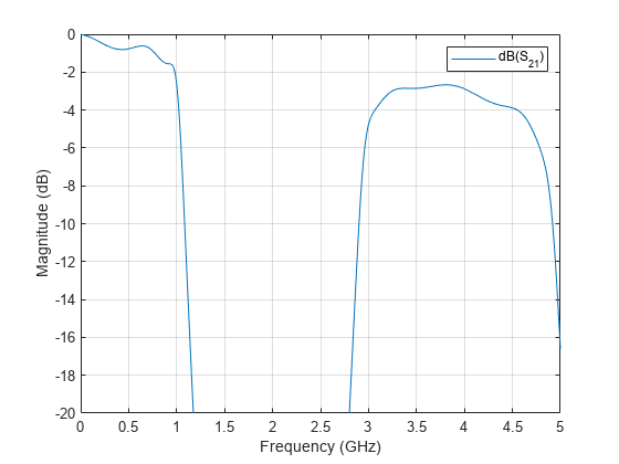
Supporting Functions
tableCircuitProperties:
type("tableCircuitProperties.m")function tableCircuitProperties(ckt,varargin)
c = cell(numel(ckt.Elements),nargin-1);
for col = 1:nargin-1
c(:,col) = {ckt.Elements.(varargin{col})};
end
disp(cell2table(c, 'VariableNames',varargin));
end
See Also
richards | kuroda | insertUnitElement | realize | txlineElectricalLength