Bandpass Filter Response Using RFCKT Objects

This example shows how to compute the time-domain response of a simple bandpass filter:

1. Choose inductance and capacitance values using the classic image parameter design method.

2. Use rfckt.seriesrlc, rfckt.shuntrlc, and rfckt.cascade objects to programmatically construct a Butterworth circuit as a 2-port network.

3. Use analyze to extract the S-parameters of the 2-port network over a wide frequency range.

4. Use s2tf function to compute the voltage transfer function from the input to the output.

5. Use rationalfit function to generate rational fits that capture the ideal RC circuit to a very high degree of accuracy.

6. Create a noisy input voltage waveform.

7. Use timeresp function to compute the transient response to a noisy input voltage waveform.

Design Bandpass Filter by Image Parameters

The image parameter design method is a framework for analytically computing the values of the series and parallel components in passive filters. For more information on this method, see "Complete Wireless Design" by Cotter W. Sayre, McGraw-Hill 2008 p. 331.

Figure 1: A Butterworth bandpass filter built out of two half-sections.

The following MATLAB® code generates component values for a bandpass filter with a lower 3-dB cutoff frequency of 2.4 GHz and an upper 3 dB cutoff frequency of 2.5 GHz.

Ro = 50;
f1C = 2400e6;
f2C = 2500e6;

Ls = (Ro / (pi*(f2C - f1C)))/2;
Cs = 2*(f2C - f1C)/(4*pi*Ro*f2C*f1C);

Lp = 2*Ro*(f2C - f1C)/(4*pi*f2C*f1C);
Cp = (1/(pi*Ro*(f2C - f1C)))/2;

Programmatically Construct Circuit as 2-Port Network

The L and C building blocks are formed by selecting appropriate values with the rfckt.shuntrlc object shown in Figure 2 or the rfckt.seriesrlc object shown in Figure 3. The building blocks are then connected together with rfckt.cascade as shown in Figure 4.

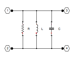
Figure 2: The 2-port network created by the rfckt.shuntrlc object

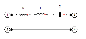
Figure 3: The 2-port network created by the rfckt.seriesrlc object

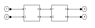
Figure 4: Connecting 2-port networks with the rfckt.cascade object

Seg1 = rfckt.seriesrlc('L',Ls,'C',Cs);
Seg2 = rfckt.shuntrlc('L',Lp,'C',Cp);
Seg3 = rfckt.shuntrlc('L',Lp,'C',Cp);
Seg4 = rfckt.seriesrlc('L',Ls,'C',Cs);

cktBPF = rfckt.cascade('Ckts',{Seg1,Seg2,Seg3,Seg4});

Extract S-Parameters From 2-Port Network

The analyze function extracts the S-parameters from a circuit over a specified vector of frequencies. This example provides a set of frequencies that spans the passband of the filter and analyzes with the default 50-Ohm reference, source impedance, and load impedances. Next, the s2tf function computes the voltage transfer function across the S-parameter model of the circuit. Finally, we generate a high-accuracy rational approximation using the rationalfit function. The resulting approximation matches the network to machine accuracy.

freq = linspace(2e9,3e9,101);
analyze(cktBPF,freq);
sparams = cktBPF.AnalyzedResult.S_Parameters;
tf = s2tf(sparams);
fit = rationalfit(freq,tf);

Verify that Rational Fit Tends to Zero

Use the freqresp function to verify that the rational fit approximation has reasonable behavior outside both sides of the fitted frequency range.

widerFreqs = linspace(2e8,5e9,1001);
resp = freqresp(fit,widerFreqs);

figure
semilogy(freq,abs(tf),widerFreqs,abs(resp),'--','LineWidth',2)
xlabel('Frequency (Hz)')
ylabel('Magnitude')
legend('data','fit')
title('The rational fit behaves well outside the fitted frequency range.')

Construct Input Signal to Test Band Pass Filter

This bandpass filter should be able to recover a sinusoidal signal at 2.45 GHz that is made noisy by the inclusion of zero-mean random noise and a blocker at 2.35 GHz. The following MATLAB code constructs such a signal from 4096 samples.

fCenter = 2.45e9;
fBlocker = 2.35e9;
period = 1/fCenter;
sampleTime = period/16;
signalLen = 8192;
t = (0:signalLen-1)'*sampleTime; % 256 periods

input = sin(2*pi*fCenter*t);     % Clean input signal
rng('default')
noise = randn(size(t)) + sin(2*pi*fBlocker*t);
noisyInput = input + noise;      % Noisy input signal

Compute Transient Response to Input Signal

The timeresp function computes the analytic solution to the state-space equations defined by the rational fit and the input signal.

output = timeresp(fit,noisyInput,sampleTime);

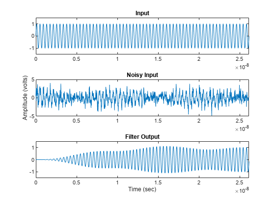
View Input Signal and Filter Response in Time Domain

Plot the input signal, noisy input signal, and the band pass filter output in a figure window.

xmax = t(end)/8;
figure
subplot(3,1,1)
plot(t,input)
axis([0 xmax -1.5 1.5])
title('Input')

subplot(3,1,2)
plot(t,noisyInput)
axis([0 xmax floor(min(noisyInput)) ceil(max(noisyInput))])
title('Noisy Input')
ylabel('Amplitude (volts)')

subplot(3,1,3)
plot(t,output)
axis([0 xmax -1.5 1.5])
title('Filter Output')
xlabel('Time (sec)')

View Input Signal and Filter Response in Frequency Domain

Overlaying the noisy input and the filter response in the frequency domain explains why the filtering operation is successful. Both the blocker signal at 2.35 GHz and much of the noise is significantly attenuated.

NFFT = 2^nextpow2(signalLen); % Next power of 2 from length of y
Y = fft(noisyInput,NFFT)/signalLen;
samplingFreq = 1/sampleTime;
f = samplingFreq/2*linspace(0,1,NFFT/2+1)';
O = fft(output,NFFT)/signalLen;

figure
subplot(2,1,1)
plot(freq,abs(tf),'b','LineWidth',2)
axis([freq(1) freq(end) 0 1.1])
legend('filter transfer function')
ylabel('Magnitude')

subplot(2,1,2)
plot(f,2*abs(Y(1:NFFT/2+1)),'g',f,2*abs(O(1:NFFT/2+1)),'r','LineWidth',2)
axis([freq(1) freq(end) 0 1.1])
legend('input+noise','output')
title('Filter characteristic and noisy input spectrum.')
xlabel('Frequency (Hz)')
ylabel('Magnitude (Volts)')

Related Topics

• Bandpass Filter Response
• Operations with RF Circuit Objects