Main Content

hyperbolicPenalty

Hyperbolic penalty value for a point with respect to a bounded region

Since R2021b

    Description

    p = hyperbolicPenalty(x,xmin,xmax) calculates the nonnegative (hyperbolic) penalty vector p for the point x with respect to the region bounded by xmin and xmax. p has the same dimension as x. This syntax uses the default values of 1 and 0.1 for the lambda and tau parameters of the hyperbolic function, respectively.

    example

    p = hyperbolicPenalty(___,lambda,tau) specifies both the lambda and tau parameters of the hyperbolic function. If lambda is an empty matrix its default value is used. Likewise if tau is an empty matrix or it is omitted, its default value is used instead.

    example

    Examples

    collapse all

    This example shows how to use hyperbolicPenalty to calculate the hyperbolic penalty for a given point with respect to a bounded region.

    Calculate the penalty value for the point 0.1 within the interval [-2,2], using default values for the lambda and tau parameters.

    hyperbolicPenalty(0.1,-2,2)
    ans = 
    0.0050
    

    Calculate the penalty value for the point 4 outside the interval [-2,2].

    hyperbolicPenalty(4,-2,2)
    ans = 
    4.0033
    

    Calculate the penalty value for the point 0.1 within the interval [-2,2], using a lambda parameter of 5.

    hyperbolicPenalty(0.1,-2,2,5)
    ans = 
    0.0010
    

    Calculate the penalty value for the point 4 outside the interval [-2,2], using a lambda parameter of 5.

    hyperbolicPenalty(4,-2,2,5)
    ans = 
    20.0007
    

    Calculate the penalty value for the point 4 outside the interval [-2,2], using a tau parameter of 0.5.

    hyperbolicPenalty(4,-2,2,5,0.5)
    ans = 
    20.0167
    

    Calculate the penalty value for the point [-2,0,4] with respect to the box defined by the intervals [0,1], [-1,1], and [-2,2] along the x, y, and z dimensions, respectively, using the default value for lambda and a tau parameter of 0.

    hyperbolicPenalty([-2 0 4],[0 -1 -2],[1 1 2],1,0)
    ans = 3×1
    
         4
         0
         4


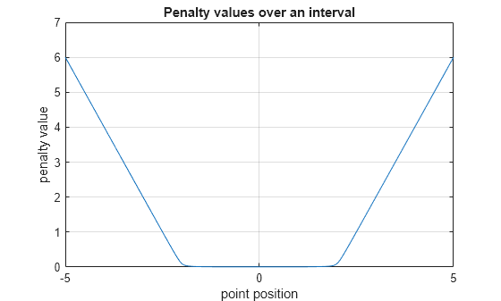
    Visualize Penalty Values for an Interval

    Create a vector of 1001 equidistant points distributed between -5 and 5.

    x = -5:0.01:5;

    Calculate penalties for all the points in the vector, using default values for the lambda and tau parameters.

    p = hyperbolicPenalty(x,-2,2);

    Plot the points and add grid, labels and title.

    plot(x,p)
    grid
    xlabel("point position");
    ylabel("penalty value");
    title("Penalty values over an interval");

    Figure contains an axes object. The axes object with title Penalty values over an interval, xlabel point position, ylabel penalty value contains an object of type line.

    Input Arguments

    collapse all

    Point for which the penalty is calculated, specified as a numeric scalar, vector or matrix.

    Example: [0.5; 1.6]

    Lower bounds for x, specified as a numeric scalar, vector or matrix. To use the same minimum value for all elements in x specify xmin as a scalar.

    Example: -1

    Upper bounds for x, specified as a numeric scalar, vector or matrix. To use the same maximum value for all elements in x specify xmax as a scalar.

    Example: 2

    Lambda parameter of the hyperbolic function, specified as a scalar.

    Example: 3

    Tau parameter of the hyperbolic function, specified as a scalar.

    Example: 0.3

    Output Arguments

    collapse all

    Penalty value, returned as a vector of nonnegative elements. Each element pi depends on the position of xi with respect to the interval specified by xmini and xmaxi. The hyperbolic penalty function returns the value:

    p(x)=λ(xxmin)+λ2(xxmin)2+τ2λ(xmaxx)+λ2(xmaxx)2+τ2

    Here, λ is the argument lambda, and τ is the argument tau. Note that for positive values of τ the returned penalty value is always positive, because on the right side of the equation the magnitude of the second term is always greater than that of the first, and the magnitude of the fourth term is always greater than that of the third. If τ is zero, then the returned penalty is zero inside the interval defined by the bounds, and it grows linearly with x outside this interval. If x is multidimensional, then the calculation is applied independently on each dimension. Penalty functions are typically used to generate negative rewards when constraints are violated, such as in generateRewardFunction.

    Extended Capabilities

    C/C++ Code Generation
    Generate C and C++ code using MATLAB® Coder™.

    Version History

    Introduced in R2021b

    Go to top of page