Modeling Target Position Errors Due to Refraction

Since R2021b

A radar system does not operate in isolation. The performance of a radar system is closely tied to the environment in which it operates. This example will discuss some of the environmental factors that are outside of the system designer's control. These environmental factors can result in losses, as well as errors in target parameter estimation.

This example first reviews several atmospheric models. Next, it presents an approximation of the standard atmospheric model using a simple exponential decay versus height. It then discusses these models within the context of a maximum range assessment and visualization of the refracted path. Lastly, it ends with a discussion on how the atmosphere causes errors in determining target height, slant range, and angle.

Atmospheric Models

Calculating tropospheric losses and the refraction phenomenon requires models of the atmospheric temperature, pressure, and water vapor density, which are dependent on height. The function atmositu offers six ITU reference atmospheric models, namely:

• Standard atmospheric model, also known as the Mean Annual Global Reference Atmosphere (MAGRA)

• Summer high latitude model (higher than 45 degrees)

• Winter high latitude model (higher than 45 degrees)

• Summer mid latitude model (between 22 and 45 degrees)

• Winter mid latitude model (between 22 and 45 degrees)

• Low latitude model (smaller than 22 degrees)

Note that for low latitudes, seasonal variations are not significant. Plot the temperature, pressure, and water vapor density profiles over a range of heights from the surface to 100 km for the default standard atmospheric model.

% Standard atmosphere model
hKm = 0:100;
h = hKm.*1e3; 
[T,P,wvden] = atmositu(h);

% Plot temperature profile
figure
subplot(1,3,1)
plot(T,hKm,'LineWidth',2)
grid on
xlabel('Temperature (K)')
ylabel('Altitude (km)')

% Plot pressure profile
subplot(1,3,2)
semilogx(P,hKm,'LineWidth',2)
grid on
xlabel('Pressure (hPa)')
ylabel('Altitude (km)')

% Plot water vapor density profile
subplot(1,3,3)
semilogx(wvden,hKm,'LineWidth',2)
grid on
xlabel('Water Vapor Density (g/m^3)')
ylabel('Altitude (km)')

% Add title
sgtitle('Standard: ITU Reference Atmosphere')

Once you have the temperature $\mathit{T}$(K), pressure $\mathit{P}$ (hPa), and water vapor density $\rho$(g/m$${}^3$$) profiles, convert these profiles to refractivity values $\mathit{N}$ as

$\mathit{N}=77.6\frac{\mathit{P}}{\mathit{T}}-5.6\frac{\mathit{e}}{\mathit{T}}+3.75\times {10}^5\frac{\mathit{e}}{{\mathit{T}}^2}$,

where $\mathit{e}$ is the water vapor pressure (hPa) calculated as

$\mathit{e}=\frac{\rho \mathit{T}}{216.7}$.

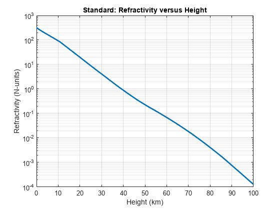
The refractivity profile for the standard atmosphere is shown here and is obtained from the function refractiveidx. refractiveidx allows you to specify one of the ITU reference models listed earlier or import custom temperature, pressure, and water vapor density profiles.

% Standard atmosphere model refractivity
[refidxStandard,refractivityStandard] = refractiveidx(h);

% Plot standard atmosphere refractivity profile 
figure
semilogy(hKm,refractivityStandard,'LineWidth',2)
grid on
xlabel('Height (km)')
ylabel('Refractivity (N-units)')
title('Standard: Refractivity versus Height')

Exponential Approximation

The Central Radio Propagation Laboratory (CRPL) developed a widely used reference atmosphere model that approximates the refractivity profile as an exponential decay versus height. This exponential decay is modeled as

$\mathit{N}={\mathit{N}}_{\mathit{S}}\exp \left(-{\mathit{c}}_{\mathit{e}}\mathit{h}\right)$,

where ${\mathit{N}}_{\mathit{S}}$ is the surface refractivity, $\mathit{h}$ is the height, and ${\mathit{c}}_{\mathit{e}}$ is a decay constant calculated as

${\mathit{c}}_{\mathit{e}}=\ln \frac{{\mathit{N}}_{\mathit{S}}}{{\mathit{N}}_{\mathit{S}}-\Delta \mathit{N}}$.

In the above equation, $\Delta \mathit{N}$is the difference between the surface refractivity ${\mathit{N}}_{\mathit{S}}$ and the refractivity at a height of 1 km. $\Delta \mathit{N}$can be approximated by an exponential function expressed as

$\Delta \mathit{N}=7.32\exp \left(0.005577{\mathit{N}}_{\mathit{S}}\right)$.

Assume the surface refractivity is 313. Calculate the decay constant using the refractionexp function. Compare the CRPL exponential model with the ITU standard atmosphere model. Note how well the two models match.

% CRPL reference atmosphere
Ns = 313; % Surface refractivity (N-units)
rexp = refractionexp(Ns); % 1/km
refractivityCRPL = Ns*exp(-rexp*hKm);

% Compare ITU and CRPL reference atmosphere models
figure
semilogy(hKm,refractivityStandard,'LineWidth',2)
grid on
hold on
semilogy(hKm,refractivityCRPL,'--r','LineWidth',2)
legend('Standard','CRPL')
xlabel('Height (km)')
ylabel('Refractivity (N-units)')
title('Refractivity versus Height')

The CRPL reference exponential model forms the basis for the blakechart function, as well as its supporting functions height2range, height2grndrange, and range2height.

Vertical Coverage

A vertical coverage pattern, also known as a Blake chart or range-height-angle chart, is a detection or constant-signal-level contour that is a visualization of refraction and the interference between the direct and ground-reflected rays. Normal atmospheric refraction is included by using an effective Earth radius and the axes of the Blake chart are built using the CRPL exponential reference atmosphere. Scattering and ducting are assumed to be negligible. The propagated range exists along the x-axis, and the height relative to the origin of the ray is along the y-axis.

To create the Blake chart, compute an appropriate free space range. Consider the case of an X-band radar system operating in an urban environment.

% Radar parameters
freq = 10e9;        % X-band frequency (Hz) 
anht = 20;          % Height (m) 
ppow = 100e3;       % Peak power (W)
tau  = 200e-6;      % Pulse width (sec)
elbw = 10;          % Half-power elevation beamwidth (deg)
Gt   = 30;          % Transmit gain (dB) 
Gr   = 20;          % Receive gain (dB)
nf   = 2;           % Noise figure (dB)
Ts   = systemp(nf); % System temperature (K)
L    = 1;           % System losses
el0  = 0.2;         % Initial elevation angle (deg) 
N    = 10;          % Number of pulses coherently integrated    
pd   = 0.9;         % Probability of detection
pfa  = 1e-6;        % Probability of false alarm 

% Surface
[hgtsd,beta0] = landroughness('Urban'); 
epsc = 5.3100 - 0.3779i; % Permittivity for concrete at 10 GHz

Assume a Swerling 1 target with a 1 m$${}^2$$ radar cross section (RCS). Determine the minimum detectable signal-to-noise ratio (SNR) using the detectability function, and then calculate the maximum detectable range using the radareqrng function. The calculated range will be used as the free space range input for radarvcd.

% Calculate coherent integration gain
Gc = pow2db(N); 

% Calculate minimum detectable SNR
minsnr = detectability(pd,pfa,10,'Swerling1') - Gc;
fprintf('Minimum detectable SNR = %.1f dB\n',minsnr);

Minimum detectable SNR = 3.5 dB

% Calculate the maximum free space range
lambda = freq2wavelen(freq); 
rcs = 1; 
maxRngKm = radareqrng(lambda,minsnr,ppow,tau, ... 
        'gain',[Gt Gr],'rcs',rcs,'Ts',Ts,'Loss',L)*1e-3; 
fprintf('Maximum detectable range in free space = %.1f km\n',maxRngKm);

Maximum detectable range in free space = 84.3 km

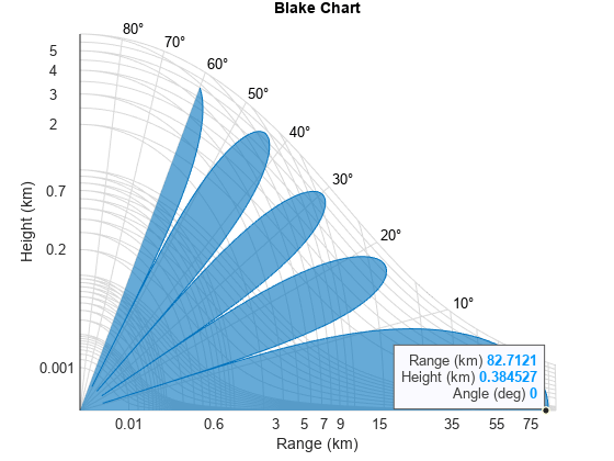
Use the radarvcd and blakechart functions in conjunction to visualize the vertical coverage of the radar system in the presence of refraction and interference between the direct and ground reflected rays. The Blake chart's constant signal level in this case is the previously calculated minimum SNR. The lobing that is seen in the following figure is the interference pattern created from the interaction of the direct and ground-reflected rays.

% Obtain the vertical coverage contour
[vcpkm,vcpang] = radarvcd(freq,maxRngKm,anht, ... 
    'SurfaceHeightStandardDeviation',hgtsd,...
    'SurfaceSlope',beta0,...
    'SurfaceRelativePermittivity',epsc,...
    'TiltAngle',el0,...
    'ElevationBeamwidth',elbw);

% Plot the vertical coverage contour on a Blake chart
figure
blakechart(vcpkm,vcpang)

Understanding Different Atmospheric Assumptions

The following section shows you how to estimate the target height under the following assumptions:

• No refraction

• Effective Earth approximation

• CRPL reference atmosphere

No Refraction

In this case, the Earth's radius is the true radius. The refractive index in this case would be equal to 1. This case presents an upper bound on the estimated target height.

% Target height assuming no refraction
Rm = linspace(0.1,maxRngKm,1000)*1e3;
Rkm = Rm*1e-3; 
Rearth = physconst('EarthRadius'); % Earth radius (m)
tgthtNoRef = range2height(Rm,anht,el0,'EffectiveEarthRadius',Rearth); 
fprintf('Target height for no refraction case %.1f m\n',tgthtNoRef(end));

Target height for no refraction case 872.7 m

Effective Earth

The effective Earth model approximates the refraction phenomena by performing calculations with an effective radius rather than the true radius. Typically, the effective Earth radius is set to 4/3 the true Earth radius.

The 4/3 Earth model suffers from two major shortcomings:

• The 4/3 Earth value is only applicable for certain areas and at certain times of the year.

• The gradient of the refractive index implied by the 4/3 Earth model is nearly constant and decreases with height at a uniform rate. Thus, values can reach unrealistically low values.

To improve the accuracy of the effective Earth calculations, you can avoid the aforementioned pitfalls by setting the effective Earth radius to a value that is more consistent with the local atmospheric conditions. For instance, if a location has a typical gradient of refractivity of $-$100 N-units/km, the effective Earth's radius factor is about 11/4 and the radius is 17,500 km.

The effearthradius function facilitates the calculation of the effective Earth radius and the corresponding fractional factor using two methods based on either the:

• Refractivity gradient, or

• An average radius of curvature calculation that considers the range, the antenna height, and the target height.

All functions that accept an effective Earth radius input can be updated with the effearthradius output to be more consistent with local conditions or the target geometry. For this example, continue with the standard 4/3 Earth.

tgthtEffEarth = range2height(Rm,anht,el0); 
fprintf('Target height for 4/3 effective Earth case %.1f m\n',tgthtEffEarth(end));

Target height for 4/3 effective Earth case 734.0 m

CRPL Reference Atmosphere

Lastly is the CRPL reference atmosphere. This is a refractivity profile that approximates the atmosphere with a decaying exponential.

tgthtCRPL = range2height(Rm,anht,el0,'Method','CRPL'); 
fprintf('Target height for CRPL case %.1f m\n',tgthtCRPL(end));

Target height for CRPL case 716.4 m

As was seen, the resulting target heights can vary greatly depending on the atmospheric assumptions.

Assuming the CRPL atmosphere is a close representation of the true atmosphere, the errors between the effective Earth radius and the CRPL method are as follows.

% Calculate true slant range and true elevation angle
[~,trueSR,trueEl] = height2range(tgthtCRPL,anht,el0,'Method','CRPL'); 

% Display errors 
fprintf('Target height error = %.4f m\n',tgthtEffEarth(end) - tgthtCRPL(end));

Target height error = 17.5602 m

fprintf('Target slant range error = %.4f m\n',Rm(end) - trueSR(end));

Target slant range error = 25.3316 m

fprintf('Target angle error = %.4f deg\n',el0 - trueEl(end));

Target angle error = 0.1059 deg

Visualizing Refraction

Next, visualize the refraction geometry including the:

• Initial ray: This is the ray as it leaves the antenna at the initial elevation angle. This would be the path of the ray if refraction was not present.

• Refracted ray: The refracted ray is the actual path of the ray that bends as it propagates through the atmosphere.

• True slant range: This is the true slant range from the antenna to the target.

• Horizontal: This is the horizontal line at the origin, coming from the antenna.

% Plot initial ray
anhtKm = anht*1e-3; 
[Xir,Yir] = pol2cart(deg2rad(el0),Rkm);
Yir = Yir + anhtKm;
figure
plot(Xir,Yir,'-.k','LineWidth',1) 
grid on
hold on

% Plot refracted ray
[X,Y] = pol2cart(deg2rad(trueEl),trueSR*1e-3);
Y = Y + anhtKm;
co = colororder; 
plot(X,Y,'Color',co(1,:),'LineWidth',2)

% Plot true slant range
X = [0 X(end)];
Y = [anhtKm Y(end)];
plot(X,Y,'Color',co(1,:),'LineStyle','--','LineWidth',2) 

% Plot horizontal line
yline(anhtKm,'Color','k','LineWidth',1,'LineStyle','-')

% Add labels
title('Refraction Geometry')
xlabel('X (km)')
ylabel('Y (km)')
legend('Initial Ray','Refracted Ray','True Slant Range', ...
    'Horizontal at Origin','Location','Best')

Target Parameter Estimation Errors

Continuing further with concepts investigated in the previous section, this section will investigate target parameter estimation errors within the context of a ground-based radar system. As was done previously, proceed from the assumption that the CRPL atmosphere is representative of the true atmosphere. Calculate the errors in height, slant range, and angle when using the 4/3 effective Earth approximation.

% Analysis parameters
tgthtTrue = 1e3;     % True target height (m)
el        = 90:-1:1; % Initial elevation angle (degrees)
anht      = 10;      % Antenna height (m)

First, calculate the propagated range, R. This is the actual refracted path of the ray through the atmosphere. The radar system would assume that the R values are the true straight-line ranges to the target and that the initial elevation angles el are the true elevation angles. However, the true slant range and elevation angles are given in the outputs trueSR and trueEl.

% Calculate the propagated range
[R,trueSR,trueEl] = height2range(tgthtTrue,anht,el,'Method','CRPL');

Next, calculate the target height under the 4/3 effective Earth radius. Plot the errors.

% Calculate target height assuming 4/3 effective Earth radius
tgtht = range2height(R,anht,el);

% This is the difference between the target height under an assumption of a
% 4/3 Earth versus what the target height truly is. 
figure
subplot(3,1,1);
plot(el,tgtht - tgthtTrue,'LineWidth',1.5) 
grid on
xlabel('Initial Elevation Angle (deg)')
ylabel(sprintf('Height\nError (m)'))

% This is the difference between the propagated range (what the radar
% detects as the range) versus what the actual true slant range is. 
subplot(3,1,2)
plot(el,(R - trueSR),'LineWidth',1.5)
grid on
xlabel('Initial Elevation Angle (deg)')
ylabel(sprintf('Range\nError (m)'))

% This is the difference between the local elevation angle (i.e., the radar
% transmitter angle) and the actual angle to the target. 
subplot(3,1,3)
plot(el,el - trueEl,'LineWidth',1.5)
grid on
xlabel('Initial Elevation Angle (deg)')
ylabel(sprintf('Angle\nError (deg)'))
sgtitle('Errors')

Note that the errors are at their worst when the initial elevation angle is small. In this case, however, since the heights of the platforms are still rather low, the effective Earth radius is a good approximation when the elevation angles are larger.

Investigating General Error Trends Due to Refraction

Calculate the height errors for different slant ranges and target heights. Consider target heights in the range from 1 m to 30 km and slant ranges from 1 m to 100 km. Convert the slant ranges to propagated range using the slant2range function. Continue to use the default CRPL parameters. After the propagated range and initial elevation angle of the propagated path is calculated, use the range2height function with the true Earth radius to calculate the apparent target heights given the initial elevation angle.

% Inputs
numPts  = 50;                            % Number of points 
tgtHgts = linspace(1e-3,30,numPts)*1e3;  % Target heights (m)
tgtSR   = linspace(1e-3,100,numPts)*1e3; % Range to target (m)
Rearth  = physconst('EarthRadius');      % Earth radius (m)
anht    = 10;                            % Antenna height (m)

% Initialize calculation
tgtPropPath = nan(numPts,numPts);        % Propagated target path (m) 
tgtEl = nan(numPts,numPts);              % Target elevation angles (deg)
tgtHgtsApparent = nan(numPts,numPts);    % Apparent target heights (m)
k = ones(numPts,numPts);                 % Effective Earth k 

% Estimate height errors using slant2range and range2height
[tgtSRGrid,tgtHgtsGrid] = meshgrid(tgtSR,tgtHgts);
idx = tgtSRGrid(:) >= abs(anht - tgtHgtsGrid(:));
[tgtPropPath(idx),tgtEl(idx),k(idx)] = slant2range(tgtSRGrid(idx),anht,tgtHgtsGrid(idx), ...
    'Method','CRPL');
tgtHgtsApparent(k~=1) = range2height(tgtPropPath(k~=1),anht,tgtEl(k~=1), ...
    'Method','Curved','EffectiveEarthRadius',Rearth);
tgtHgtsErr = tgtHgtsApparent - tgtHgtsGrid;

Draw contour lines to display the height error as a function of true target height and slant range. The plot indicates that at the farthest ranges and the lower target altitudes, height errors up to about 200 meters can be seen.

% Plot height error contours
figure('Name','Height Error Contours')
tgthgtErrorLevels = [2 5 10 20 30 50:25:300]; % Contour levels (m)
[~,hCon1] = contour(tgtSR*1e-3,tgtHgts*1e-3, ...
    tgtHgtsErr,tgthgtErrorLevels,'ShowText','on');
hCon1.LineWidth = 1.5;
grid on
xlabel('Slant Range (km)')
ylabel('True Target Height (km)')
hCb = colorbar;
hCb.Label.String = 'Height Errors (m)';
axis equal
title('Height Error Contours (m)')

Summary

This example discussed atmospheric models and investigated their effect on target range, height, and angle estimation.

References

1. Barton, David K. Radar Equations for Modern Radar. Norwood, MA: Artech House, 2013.

2. Blake, L.V. "Radio Ray (Radar) Range-Height-Angle Charts." Naval Research Laboratory, NRL Report 6650, Jan. 22, 1968.

3. Blake, L.V. "Ray Height Computation for a Continuous Nonlinear Atmospheric Refractive-Index Profile." RADIO SCIENCE, Vol. 3 (New Series), No. 1, Jan. 1968, pp. 85-92.

4. Bean, B. R., and G. D. Thayer. CRPL Exponential Reference Atmosphere. Washington, DC: US Gov. Print. Off., 1959.

5. International Telecommunication Union (ITU). "Attenuation by Atmospheric Gases". Recommendation ITU-R P.676-12, P Series, Radiowave Propagation, August 2019.

6. Weil, T. A. "Atmospheric Lens Effect: Another Loss for the Radar Range Equation." IEEE Transactions on Aerospace and Electronic Systems, Vol. AES-9, No. 1, Jan. 1973.