Create a Digital Twin of a TI mmWave Radar
This example creates a waveform-level model of a TI mmWave radar using the radar's configuration file, and it explains how to leverage custom RF components for simulating real systems in MATLAB® software. You will compare the synthetic data with data collected from the real-world TI radar and demonstrate the strong similarity between the actual sensor and its model.
Introduction
Radar Toolbox™ allows you to collect I/Q data from the TI mmWave radar sensors listed in Installation, Setup, and Supported Boards as demonstrated in I/Q Data Collection and Detection Generation with Texas Instruments (TI) millimeter-wave (mmWave) Radar. This example compliments the real data collection tutorial and shows, step by step, how to create an accurate model of the TI hardware and waveform using the radarTransceiver. This allows you to test your algorithm in custom scenarios without the overhead of running costly experiments.
This example considers the IWR1642BOOST automotive radar paired with a data acquisition board (DCA1000EVM). Together, these boards export raw I/Q samples that can be processed and visualized using the many functions and system objects provided in MATLAB.
Model a Radar Transceiver from the Configuration File
Read the Configuration File
In order to run the TI radar, you must first send the radar board a configuration file that specifies the waveform and the configurable properties of the hardware and software. The format and explanation of the configuration file is described in detail in the MMWAVE SDK User Guide linked in this table. The rest of the example uses the following configuration file shown below.
type("exampleConfig.cfg")sensorStop flushCfg dfeDataOutputMode 1 channelCfg 15 3 0 adcCfg 2 1 adcbufCfg -1 0 1 1 1 profileCfg 0 77 150 7 75 0 0 25 1 400 6250 0 0 30 chirpCfg 0 0 0 0 0 0 0 1 chirpCfg 1 1 0 0 0 0 0 2 frameCfg 0 1 40 0 100 1 0 lowPower 0 1 guiMonitor -1 1 1 0 0 0 1 cfarCfg -1 0 2 8 4 3 0 15 1 cfarCfg -1 1 0 8 4 4 1 15 1 multiObjBeamForming -1 1 0.5 clutterRemoval -1 0 calibDcRangeSig -1 0 -5 8 256 extendedMaxVelocity -1 0 bpmCfg -1 0 0 1 lvdsStreamCfg -1 0 1 0 compRangeBiasAndRxChanPhase 0.0 1 0 1 0 1 0 1 0 1 0 1 0 1 0 1 0 measureRangeBiasAndRxChanPhase 0 1.5 0.2 CQRxSatMonitor 0 3 4 95 0 CQSigImgMonitor 0 95 4 analogMonitor 0 0 aoaFovCfg -1 -90 90 -90 90 cfarFovCfg -1 0 0 10.00 cfarFovCfg -1 1 -2.59 2.59 calibData 0 0 0 sensorStart
Many of the lines in the configuration file are mandatory to operate the radar but are not relevant for exporting raw samples from the radar to your computer or for the waveform-level model of the radar. Instead, they configure the post processing that would be done on the radar if you wanted to export detection/measurement level data, similar to what would be exported from the radarDataGenerator. Thus, you can create an accurate model of the radar from just a few lines of the configuration file and the information contained in the radar's datasheets.
The relevant lines in the configuration file are:
Line Header | Description |
| Determines the waveform and analog to digital converter (ADC) properties |
| Determines the variations between each chirp or pulse (if any) |
| Determines how many chirps are in each frame (also known as a coherent processing interval, CPI) and how many frames are transmitted |
For more information, explore the following links:
Link | Description |
MMWAVE SDK User Guide (Configuration File) | |
IWR1642 datasheet (Just the Chip) | |
IWR1642BOOST datasheet (Evaluation Board) |
Parsing the configuration file by referring to the MMWAVE SDK User Guide can be tedious, especially if you are still changing and/or comparing different configurations. To help simplify the process, a helper class is provided to parse the relevant lines in the configuration file.
Parse the configuration with the following helper class.
radarCfg = helperParseRadarConfig("exampleConfig.cfg")radarCfg =
helperParseRadarConfig with properties:
StartFrequency: 7.7000e+10
StopFrequency: 7.8875e+10
CenterFrequency: 7.7938e+10
Bandwidth: 1.6000e+09
SampledRampTime: 6.4000e-05
ChirpCycleTime: 2.2500e-04
SweepSlope: 2.5000e+13
SamplesPerChirp: 400
ADCSampleRate: 6250000
NumChirps: 80
NumReceivers: 4
ActiveReceivers: 4
NumTransmitters: 2
ActiveTransmitters: 2
FramePeriodicity: 0.1000
RangeResolution: 0.0937
MaximumRange: 37.4741
MaximumRangeRate: 2.1370
RangeRateResolution: 0.1068
RxGain: 30
PRF: 4.4444e+03
This helper class assumes the use of time division multiplexing (TDM) by alternating between the two transmitting antennas for each chirp. Moreover, the helper class assumes that every transmitted chirp's waveform is identical. As a result, the chirpCfg lines can be ignored. Furthermore, this parser assumes that all receivers are enabled. Modify the parser class to support changing these features as well as other configurable features not contained in the parsed lines.
Once the radar configuration file is parsed, use the helperRadarAndProcessor class to create the accompanying radar transceiver and associated processing blocks, such as the range-Doppler processor and CFAR detector.
addpath("tiRadar")
radarSystem = helperRadarAndProcessor(radarCfg)
radarSystem =
helperRadarAndProcessor with properties:
RadarTransceiver: [1×1 radarTransceiver]
AntennaNoiseCfg: []
VirtualArray: [1×1 phased.ULA]
Fc: 7.7938e+10
Fs: 1.6000e+09
NumSamplesDuringPulseWidth: 102400
RangeDopplerProcessor: [1×1 phased.RangeDopplerResponse]
RangeProcessor: [1×1 phased.RangeResponse]
PhaseShiftBf: [1×1 phased.PhaseShiftBeamformer]
TwoDimCFAR: [1×1 phased.CFARDetector2D]
The radar transceiver itself is contained in the RadarTransceiver property of the object as shown immediately below. The next few sections outline how the helperRadarAndProcessor's radarTransceiver System Object™ is designed to match the TI radar.
radarSystem.RadarTransceiver
ans =
  radarTransceiver with properties:

                Waveform: [1×1 phased.LinearFMWaveform]
             Transmitter: [1×1 phased.Transmitter]
         TransmitAntenna: [1×1 phased.Radiator]
          ReceiveAntenna: [1×1 phased.Collector]
                Receiver: [1×1 phased.Receiver]
      MechanicalScanMode: 'None'
      ElectronicScanMode: 'None'
        MountingLocation: [0 0 0]
          MountingAngles: [0 0 0]
    NumRepetitionsSource: 'Property'
          NumRepetitions: 1
       RangeLimitsSource: 'Property'
             RangeLimits: [0 Inf]
         RangeOutputPort: false
          TimeOutputPort: false
Configure the Antennas
Antenna Arrays
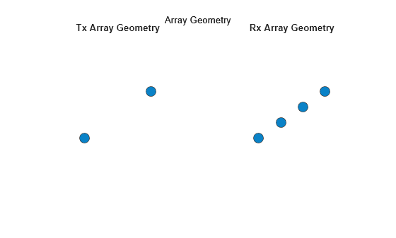
There are two antenna arrays on the IWR1642BOOST, one for transmitting and one for receiving. The transmit antenna array contains two antenna elements spaced two wavelengths apart from each other. The receiving antenna array consists of four antenna elements each spaced half of a wavelength apart. They are each visualized below.
figure;
subplot(1,2,1)
viewArray(radarSystem.RadarTransceiver.TransmitAntenna.Sensor,'ShowLocalCoordinates',false,'ShowAnnotation',false)
title('Tx Array Geometry')
subplot(1,2,2)
viewArray(radarSystem.RadarTransceiver.ReceiveAntenna.Sensor,'ShowLocalCoordinates',false,'ShowAnnotation',false)
title('Rx Array Geometry')
Using TDM, the transmit and receive antenna arrays manifest into the following virtual array. More about creating large virtual arrays can be found in Simulate an Automotive 4D Imaging MIMO Radar
figure;
viewArray(radarSystem.VirtualArray)
title('Virtual Array')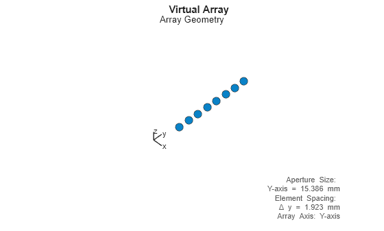
Antenna Elements
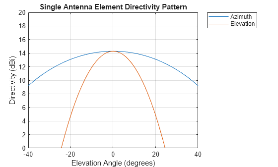
Both antenna arrays are made of elements modeled by the phased.CosineAntennaElement system object. This serves as an approximation of the directivity pattern measured and is documented in the IWR1642BOOST datasheet linked above. Other antenna element models are also available in the Phased Array System Toolbox™. For the most precise modeling of the antenna elements' directivity, use the phased.CustomAntennaElement and model the exact gain patterns plotted in the documentation. For the cosine approximation, the directivity pattern near boresight was prioritized in this approximation leading to a mismatch in the peak gain at boresight. You can remove this by changing the exponents of the cosine antenna elements or by adding an amplifier with a negative gain in the transmitter described in the next section. However, with the goal of matching the SNR of the actual device, you can also wait and apply only the net SNR difference with the actual model after all such approximations, if there is any. This comparison is shown in Compare Synthetic and Real-World Data. Display the antenna element patterns below using the pattern method.
element = radarSystem.RadarTransceiver.TransmitAntenna.Sensor.Element;

figure;
az = -180:180;
el = 0;
pattern(element,radarCfg.CenterFrequency,az,el,CoordinateSystem="rectangular",Type='directivity');
hold on;
az = 0;
el = -90:90;
pattern(element,radarCfg.CenterFrequency,az,el,CoordinateSystem="rectangular",Type='directivity');
legend('Azimuth','Elevation')
title('Single Antenna Element Directivity Pattern')
xlim([-40 40])
ylim([0 20])
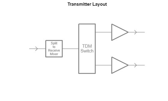
Transmitter
The transmitter in the radar transceiver accounts for three main features of the TI radar:
Signal Splitter (for dechirping on the receive end)
Time Division Multiplexing (alternating between elements in the transmit antenna array)
Transmitted Power
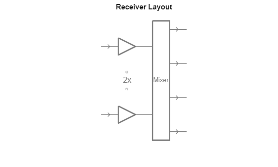
These features are implemented using the cascade transmitter/receiver design depicted below.
figure
viewLayout(radarSystem.RadarTransceiver.Transmitter)
Signal Splitter
The radar processes reflected signals first by mixing them with the transmitted waveform (instead of matched filtering). To implement this mixing operation, use the signal splitter in the transmitter to feed a copy of the transmitted waveform to the receiver and then to a custom mixer in the receiver.
Time Division Multiplexing
The code in the directory tiRadar implements a custom object that switches the active transmit antenna for each chirp. The logic that accomplishes this is inside the step implementation in helperTDMSwitch.m. The step implementation creates a matrix of zeros of size n elements by the length of the transmitted signal. During simulation, only the active column has a nonzero signal, which results in only one antenna transmitting at a time.
Transmit Power
Lastly, the transmitted power according to the IWR1642 datasheet is 12.5 dBm. Because the waveform objects have an amplitude of one, model the specified transmit power using an amplifier operating in saturation in series with the TDM switch.
transmitPower = radarSystem.RadarTransceiver.Transmitter.Cascade{3}.OPsat % dBmtransmitPower = 12.5000
Receiver
The modeled receiver accounts for the low noise amplifier (LNA) and the mixing operation.
figure
viewLayout(radarSystem.RadarTransceiver.Receiver)
Low Noise Amplifier
The first step is to apply the LNA by setting its receiver gain and the noise figure. The receiver gain is defined in the radar configuration class in the RxGain property, and the noise figure is set to 15 dB according to the IWR1642 datasheet. Additionally, according to the IWR1642 documentation, the receiver subsystem can support bandwidths of up to 5 MHz so the sample rate is set accordingly to approximate the noise bandwidth.
LNA = radarSystem.RadarTransceiver.Receiver.Cascade{1};
rxGain = LNA.Gain
rxGain = 30
noiseFigure = LNA.NF
noiseFigure =
15
receiverNoisebandwidth = LNA.SampleRate
receiverNoisebandwidth =
5000000
Mixer
The mixer performs the dechirping necessary to compute the range of the target reflections. Dechirping refers to the mixing of the incoming reflected signal with the transmitted signal. This is an alternative to matched filtering and allows for a lower bandwidth receiver than matched filtering would enable. The mixer mixes the amplified received signal with a copy of the transmitted waveform.
Waveform
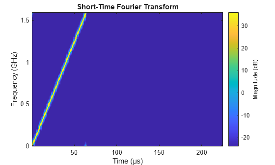
The TI radar transmits a linear frequency modulated waveform. While both the phased.LinearFMWaveform and phased.FMCWWaveform create such waveforms, only the LFM waveform System Object models duty cycles less than 100%. According to the configuration, there is a chirp every 225 microseconds while the sampled ramp time is only 64 microseconds, yielding a duty cycle of about 28%. In other words, the waveform is only active approximately 28% of the total PRI. This does not account for the over sweep [1] present in the waveform.
PRI = 1/radarCfg.PRF
PRI =
2.2500e-04
sampledRampTime = radarCfg.SampledRampTime
sampledRampTime =
6.4000e-05
dutyCycle = sampledRampTime/PRI
dutyCycle =
0.2844
Given this waveform design, configure the LFM waveform with a ramp time equal to the sampled ramp time and with the rest of the PRI without any signal transmission as shown in the figure below.
figure
stft(radarSystem.RadarTransceiver.Waveform(),radarSystem.Fs,'FrequencyRange','twosided')
Sampling Rate
The real TI hardware includes an analog front end that mixes down the signal to an intermediate frequency (IF) proportional to the reflections' ranges. This allows the hardware to sample at a rate much lower than the bandwidth of the waveform. In this software simulation, we construct a digital representation of the waveform and thus need to sample this waveform at its bandwidth. Thus, the LFM waveform, which has a bandwidth of 1.6 GHz must be sampled at 1.6 GHz. Only after creating the high-bandwidth digital waveform and receiving target reflections can it be mixed down to its IF frequencies. However, we can still simulate data sampled at the proper rate (one that matches the actual radar hardware) by downsampling the IF signal after the mixing operation using the downsampleIF method. You demonstrate this in the next section.
Number of Chirps/Pulses
The number of chirps per frame can be configured in three separate places. The correct place to configure this property depends on the nature of the application and is described below.
When analyzing the waveform object by itself, set the number of chirps in the waveform system object to the desired value. For example, in
phased.LinearFMWaveform, modify theNumPulsesproperty.In most general cases when using a
radarTransceiver, set theradarTransceiverNumRepetitionsproperty to the desired number of chirps. This is applicable when the velocity is constant within a frame or CPI.When using the
radarTransceiverwith targets that need to be moved or modified between chirps such as thebackscatterPedestrianandbackscatterBicyclist, keep theradarTransceiverNumRepetitionsproperty equal to one. Then step the radar transceiver in a for-loop where each iteration transmits and receives one chirp. Set the number of for loop iterations to the desired number of chirps.
Data Processing
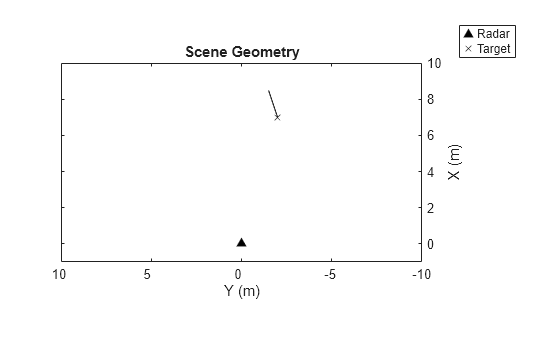
To demonstrate how the model of the IWR1642BOOST senses point targets, create a point target with a position and velocity. A point target's motion-induced phase shift is automatically accounted for between chirps so set the radar transceiver's number of repetitions to the number of chirps.
release(radarSystem.RadarTransceiver.Waveform) % Due to earlier code in example
% Use with target that does not need manual move/update between chirps
radarSystem.RadarTransceiver.NumRepetitions = radarCfg.NumChirps;
tgt1 = struct('Position', [7 -2 0], 'Velocity', [1.5 .5 0]);
Note the orientation of the y-values in the theater plot below. The axes are oriented so that the positive z-axis points out of the computer screen. Because of this, in the later plots and in the beamforming output, the target will remain on the right as it is here but will have a positive horizontal axis value.
tp = theaterPlot('XLim',[-1 10],'YLim',[-10 10]);
radarPlotter = platformPlotter(tp,'DisplayName','Radar','Marker','^','MarkerFaceColor','k');
targetPlotter = platformPlotter(tp,'DisplayName','Target','Marker','x');
plotPlatform(radarPlotter, [0 0 0])
plotPlatform(targetPlotter, tgt1.Position,tgt1.Velocity)
title('Scene Geometry')
camroll(90)
Now, simulate the transmission of the waveform and reception of the reflected signal. Remember, the step function of the radar transceiver returns the already mixed down IF signal from the target. Then, take only the samples during the active portion of the waveform and downsample them accordingly. The size of the signal after downsampling is the number of samples per chirp by the number of channels by the number of chirps per frame.
time = 0;
sig = radarSystem.RadarTransceiver(tgt1,time);
sig = radarSystem.downsampleIF(sig);
size(sig)
ans = 1×3

   400     4    80
Range-Doppler Processing
Use the method boresightRD to compute the range-Doppler response at boresight. This method reformats the datacube so that the channel dimension (dimension 2) is the same size as the virtual array (8 virtual channels). Then, it sums across the virtual channels and computes the range-Doppler response.
% RD processing
[rgdp,rngBins,dpBins] = radarSystem.boresightRD(sig);
CFAR Detection
Perform 2D-CFAR detection using the findPeaksRangeDoppler method in the radarSystem object. Extend the range-Doppler output using circular padding to allow the detection of targets near the unambiguous Doppler limits. The CFAR parameters are defined in the method Create2DCFAR in the helperRadarAndProcessor class. The detector outputs multiple detections for the point target in the configured scene. The CFAR mask on the right shows the cells tested for a target as well as the cells that returned one. The detections from the CFAR mask are further filtered so that only the strongest peak per range bin is returned. Edit the CFAR parameters and see how the detection results change.
% 2D CFAR
[cfarMask,peakLocations] = radarSystem.findPeaksRangeDoppler(rgdp);
radarSystem.cfarPlotter(rgdp,cfarMask,peakLocations,rngBins,dpBins)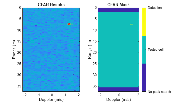
Angle Processing
Process the angle data in the horizontal plane (azimuth) using the getBfRangeAnglePatch defined in the helperRadarAndProcessor class. This custom method returns the beamforming output as well as its projection onto a cartesian coordinate system. Again, note that the convention in the theater plot above is such that the y-values are negative to the right of the radar. As a result, the peak in the beamforming output that is to the right of the origin has a positive y-value.
Moving targets detected by a radar that employs TDM can cause an abrupt phase jump between antennas 4 and 5 in the virtual array. This is because the target has moved slightly between transmissions. Simply concatenating the received signals into a virtual array does not account for the resultant phase jump and can cause error in the angle estimation of the target. Authors in [2] correct for this by upsampling the pulse dimension and then staggering the signals such that received samples alternate in the same way as the transmitting antennas. See the short implementation in the method upsampleAndStagger for more details. Try processing the angle data with and without the TDM correction.
TdmCorrection = true;
[bfOut,cartData,xBounds,yBounds,tgtAngles] = radarSystem.getBfRangeAnglePatch(sig,peakLocations,rngBins,TdmCorrection);

helperPlotBfOutput(bfOut,tgt1,xBounds,yBounds,cartData)
true;
[bfOut,cartData,xBounds,yBounds,tgtAngles] = radarSystem.getBfRangeAnglePatch(sig,peakLocations,rngBins,TdmCorrection);
helperPlotBfOutput(bfOut,tgt1,xBounds,yBounds,cartData)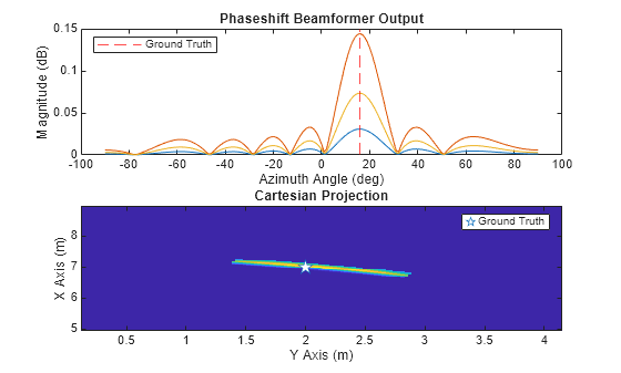
Compare Synthetic and Real-World Data
This section demonstrates the similarity between synthetic data and data collected using the TI IWR1642BOOST. To collect real data, we configured the IWR1642BOOST using the same configuration detailed in the beginning of this example. Then, we had a human move a corner reflector towards the radar. In the collected frame, the corner reflector has a range of 3.9 meters and an azimuth of 5 degrees. The target is also moving at 0.42 m/s towards the radar.
For this comparison, create a similar scene containing a point target with the same position and velocity as observed in the real-world data. Below, we show that when identical processing is applied to real-world and synthetic data, the results are very similar.
Synthetic Data
Define a corner reflector target (tgt2) and generate a synthetic datacube using the digital twin's radarTransceiver.
tgt2 = struct('Position', [3.9*cosd(5) -3.9*sind(5) 0], 'Velocity', [-.42 0 0], ...
    'Signatures',{rcsSignature(Pattern=-10)});
sig = radarSystem.RadarTransceiver(tgt2,time);
sig = radarSystem.downsampleIF(sig);

% Boresight Range-Doppler Processing
rgdpSynthetic = radarSystem.boresightRD(sig);
[M,I] = max(rgdpSynthetic,[],'all'); % find peak in range-Doppler
[rangeIdx,dopIdx] = ind2sub(size(rgdpSynthetic),I);
peakLocation = [rangeIdx; dopIdx];
normalizedMagSynthetic = mag2db(abs(rgdpSynthetic)) - max(mag2db(abs(rgdpSynthetic(:))));

% Angle Processing
polarBfSynthetic = radarSystem.getBfRangeAnglePatch(sig,peakLocation,rngBins,true);
Real-World Data
Load in real-world data collected using the same configuration file discussed above. This data has already been rearranged so that the received signals from transmitter one and transmitter two are concatenated.
realWorldRadarData = load('realDataExample.mat').movingReflectorData;Remove the static clutter from the real data so that the detected peak is made up primarily from the moving corner reflector. To remove the static clutter, subtract the mean across the slow-time dimension of the datacube.
realWorldRadarData = realWorldRadarData - mean(realWorldRadarData,3);
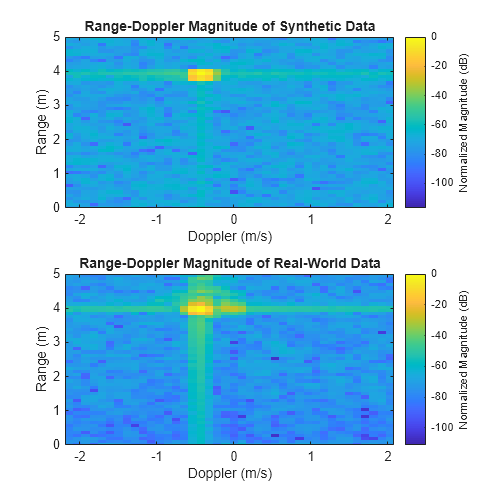
Range Doppler Processing
Apply the same radar processing as was used for the synthetic data generated from the digital twin by computing the range-Doppler response after summing the received channels. Then, plot the normalized magnitude.
realWorldSigSumChannels = squeeze(sum(realWorldRadarData,2)); % beamform toward boresight
[rgdpRealWorld,rngBins,dpBins] = radarSystem.RangeDopplerProcessor(realWorldSigSumChannels);
normalizedMagRealWorld = mag2db(abs(rgdpRealWorld)) - max(mag2db(abs(rgdpRealWorld(:))));
Plot the normalized magnitude of the range-Doppler response for both the synthetic and the real radar data.
helperCompareRangeDoppler(normalizedMagRealWorld,normalizedMagSynthetic,dpBins,rngBins)
Test the SNR of the synthetic and real data by comparing the peak value with the median value of the range-Doppler response
syntheticSNR = max(mag2db(abs(rgdpSynthetic(:)))) - median(mag2db(abs(rgdp(:))))
syntheticSNR =
72.4611
realWorldSNR = max(mag2db(abs(rgdpRealWorld(:)))) - median(mag2db(abs(rgdpRealWorld(:))))
realWorldSNR =
72.0072
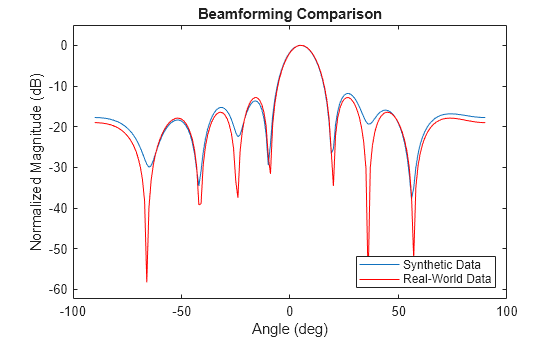
Angle Processing
Reformat the data such that the channel dimension is set to the number of receive antennas (4) and the chirps from each transmitter are interleaved with each other. Then use the getBfRangeAnglePatch method just as we did for the synthetic data. Note how similar the beamwidth and sidelobe levels are in the real and synthetic data.
realWorldRadarData = helperReformatData(realWorldRadarData);
realWorldBf = radarSystem.getBfRangeAnglePatch(realWorldRadarData,peakLocation,rngBins,true);

figure;
plot(-90:90,mag2db(realWorldBf/max(realWorldBf)))
hold on;
plot(-90:90,mag2db(polarBfSynthetic/max(polarBfSynthetic)),'r')
legend({'Synthetic Data','Real-World Data'},'Location','southeast')
xlabel('Angle (deg)')
ylabel('Normalized Magnitude (dB)')
title('Beamforming Comparison')
axis padded
Summary
This example walks you through modeling a TI mmWave radar directly from the radar's configuration file and simulates custom electronic components that model features like TDM and dechirping. It also demonstrates an example processing pipeline for the radar data. Finally, the example shows that the synthetic data matches the real-world data very closely.
References
[1] Scheer, Jim, and William A. Holm. "Principles of modern radar." (2010): 3-4.
[2] Bechter, Jonathan, Fabian Roos, and Christian Waldschmidt. "Compensation of motion-induced phase errors in TDM MIMO radars." IEEE Microwave and Wireless Components Letters 27, no. 12 (2017): 1164-1166.
Helper Functions
function dataOut = helperReformatData(dataIn)
    % put it in format such that there are only 4 channels and the chirps
    % are from alternating transmitters
    dataOut = zeros(size(dataIn,1),.5*size(dataIn,2),2*size(dataIn,3));
    dataOut(:,:,1:2:end) = dataIn(:,1:4,:);
    dataOut(:,:,2:2:end) = dataIn(:,5:end,:);
end

%% Plotting Helper Functions

function helperPlotBfOutput(bfOut,tgt1,xBounds,yBounds,cartData)
    figure;
    subplot(2,1,1)
    plot(-90:90,bfOut')
    hold on;
    gt = xline(-atand(tgt1.Position(2)/tgt1.Position(1)),'r--');
    xlabel('Azimuth Angle (deg)')
    ylabel('Magnitude (dB)')
    title('Phaseshift Beamformer Output')
    legend(gt,'Ground Truth','Location','northwest')

    subplot(2,1,2);
    imagesc(xBounds,yBounds,cartData)
    hold on;
    plot(-tgt1.Position(2),tgt1.Position(1),'pentagram','MarkerSize',10,'MarkerFaceColor','w')
    xlabel('Y Axis (m)')
    ylabel('X Axis (m)')
    title('Cartesian Projection')
    axis xy
    legend('Ground Truth')
end

function helperCompareRangeDoppler(normalizedMagRealWorld,normalizedMagSynthetic,dpBins,rngBins)
    f = figure;
    f.Position(3:4) = [500 500];
    subplot (2,1,1)
    imagesc(dpBins,rngBins,normalizedMagSynthetic);
    xlabel('Doppler (m/s)')
    ylabel('Range (m)')
    title('Range-Doppler Magnitude of Synthetic Data')
    axis xy
    ylim([0,5])
    c = colorbar;
    c.Label.String = 'Normalized Magnitude (dB)';
    subplot(2,1,2)
    imagesc(dpBins,rngBins,normalizedMagRealWorld);
    xlabel('Doppler (m/s)')
    ylabel('Range (m)')
    title('Range-Doppler Magnitude of Real-World Data')
    axis xy
    ylim([0,5])
    c = colorbar;
    c.Label.String = 'Normalized Magnitude (dB)';
end