Train and Test TCN Anomaly Detector

Load the file sineWaveAnomalyData.mat, which contains two sets of synthetic three-channel sinusoidal signals.

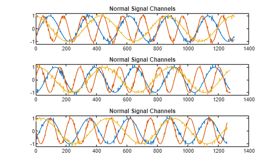
sineWaveNormal contains 10 sinusoids of stable frequency and amplitude. Each signal has a series of small-amplitude impact-like imperfections. The signals have different lengths and initial phases.

load sineWaveAnomalyData.mat sineWaveNormal sineWaveAbnormal
s1 = 3;

Plot input signals

Plot the first three normal signals. Each signal contains three input channels.

tiledlayout("vertical")
ax = zeros(s1,1);
for kj = 1:s1
    ax(kj) = nexttile;
    plot(sineWaveNormal{kj})
    title("Normal Signal Channels")
end

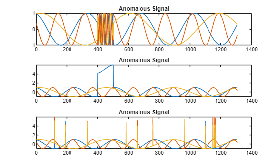
sineWaveAbnormal contains three signals, all of the same length. Each signal in the set has one or more anomalies.

• All channels of the first signal have an abrupt change in frequency that lasts for a finite time.

• The second signal has a finite-duration amplitude change in one of its channels.

• The third signal has spikes at random times in all channels.

Plot the three signals with anomalies.

tiledlayout("vertical")
ax = zeros(s1,1);
for kj = 1:s1
    ax(kj) = nexttile;
    plot(sineWaveAbnormal{kj})
    title("Anomalous Signal")
end

Create Detector

Use the tcnAD function to create a tcnDetector object with default options.

detector_tcn = tcnAD(3)

detector_tcn = 
  TcnDetector with properties:

               FilterSize: 7
       DropoutProbability: 0.2500
    DetectionWindowLength: 10
          DetectionStride: 10
               NumFilters: 32
                IsTrained: 0
              NumChannels: 3
                   Layers: [23×1 nnet.cnn.layer.Layer]
                    Dlnet: [1×1 dlnetwork]
                Threshold: []
          ThresholdMethod: 'kSigma'
       ThresholdParameter: 3
        ThresholdFunction: []
            Normalization: 'zscore'

Train Detector

Prepare to train detector_tcn by customizing a trainingOptions option set with a solver of "adam" and a limit of 100 for the number of training epochs.

trainopts = trainingOptions("adam",MaxEpochs=100);

Train detector_tcn using the normal data and trainopts.

detector_tcn = train(detector_tcn,sineWaveNormal,trainingOpts=trainopts);

    Iteration    Epoch    TimeElapsed    LearnRate    TrainingLoss
    _________    _____    ___________    _________    ____________
            1        1       00:00:00        0.001          1.6331
           50       50       00:00:03        0.001         0.13097
          100      100       00:00:06        0.001        0.085445
Training stopped: Max epochs completed
Computing threshold...
Threshold computation completed.

View the threshold that train computes and saves within detector_tcn. This computed value is influenced by random factors, such as which subsets of the data are used for training, and can change somewhat for different training sessions and different machines.

thresh = detector_tcn.Threshold

thresh = single

3.2729

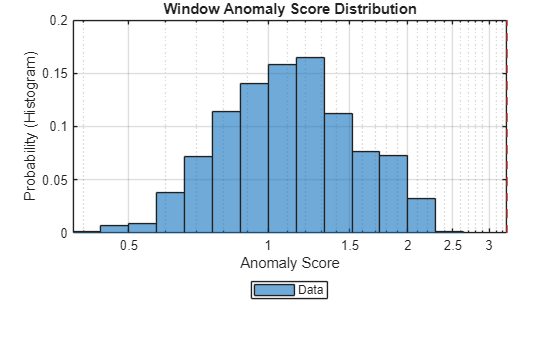
Plot the histogram of the anomaly scores for the normal data. Each score is calculated over a single detection window. The threshold, plotted as a vertical line, does not always completely bound the scores.

plotHistogram(detector_tcn,sineWaveNormal)

Use Detector to Identify Anomalies

Use the detect function to determine the anomaly scores for the anomalous data.

results = detect(detector_tcn, sineWaveAbnormal)

results=3×1 cell array
    {130×3 table}
    {130×3 table}
    {130×3 table}

results is a cell array that contains three tables, one table for each channel. Each cell table contains three variables: WindowLabel, WindowAnomalyScore, and WindowStartIndices. Confirm the table variable names.

varnames = results{1}.Properties.VariableNames

varnames = 1×3 cell
    {'WindowLabels'}    {'WindowAnomalyScores'}    {'WindowStartIndices'}

Plot Results

Plot a histogram that shows the normal data, the anomalous data, and the threshold in one plot.

plotHistogram(detector_tcn,sineWaveNormal,sineWaveAbnormal)

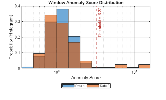
The histogram uses different colors for the normal and anomalous data.

Plot the detected anomalies of the third abnormal signal set.

plot(detector_tcn,sineWaveAbnormal{3})

The top plot shows an overlay of red where the anomalies occur. The bottom plot shows how effective the threshold is at dividing the normal from the abnormal scores for Signal set 3.