Fault Detection and Remaining Useful Life Estimation Using Categorical Data
This example shows how to create models for fault classification and remaining useful life (RUL) estimation using categorical machine data. Categorical data is data that has values in a finite set of discrete categories. For machine data, categorical variables can be the manufacturer's code, location of the machine, and experience level of the operators. You can use these variables as predictors, along with other measured sensor data, to help identify which machines will need maintenance.
Here, you use categorical variables to train a binary decision tree model that classifies if machines are broken. Then you fit a covariate survival model to the data to predict RUL.
Data Set
The data set [1] contains simulated sensor records of 999 machines made by four different providers with slight variations among their models. The simulated machines were used by three different teams over the simulation timespan. In total, the data set contains seven variables per machine:
Lifetime(numeric) — Number of weeks the machine has been activeBroken(boolean) — Machine status, where true indicates a broken machinePressureInd(numeric) — Pressure index. A sudden drop can indicate a leak.MoistureInd(numeric) — Moisture index (relative humidity). Excessive humidity can create mold and damage the equipment.TemperatureInd(numeric) — Temperature indexTeam(categorical) — Team using the machine, represented as a stringProvider(categorical) — Machine manufacturer name, represented as a string
The strings in the Team and Provider data represent categorical variables that contain nonnumeric data. Typically, categorical variables have the following forms:
String or character data types: Can be used for nominal categorical variables, where the value does not have any ranking or order
Integer or enumerated data types: Can be used for ordinal categorical variables, where the values have a natural order or ranking
Boolean data type: Can be used for categorical variables with only two values
In addition, MATLAB® provides a special data type, categorical, that you can use for machine-learning computations. The categorical command converts an array of values to a categorical array.
Load the data.
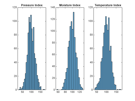
load('simulatedData.mat');Plot histograms of the numeric machine variables in the data set to visualize the variable distribution. The histograms help you assess the distribution of the values and identify outliers or unusual patterns within the data set. These histograms show that the data in pressureInd, moistureInd, and temperatureInd is normally distributed.
figure;
tiledlayout(1,3)
%
nexttile;
histogram(simulatedData.pressureInd);
title('Pressure Index');
%
nexttile;
histogram(simulatedData.moistureInd);
title('Moisture Index');
%
nexttile;
histogram(simulatedData.temperatureInd);
title('Temperature Index');

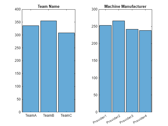
Create histograms of the categorical variables. The categorical values are well balanced.
figure;
tiledlayout(1,2)
%
nexttile;
histogram(categorical(simulatedData.team));
title('Team Name');
%
nexttile;
histogram(categorical(simulatedData.provider));
title('Machine Manufacturer');

Prepare Categorical Variables
To use categorical variables as predictors in machine learning models, you convert them to numeric representations. The categorical variables in the data set have a data type of string. MATLAB provides a special data type, categorical, that you can use for computations that are designed specifically for categorical data. The categorical command converts an array of values to a categorical array.
Once you have converted the strings to categorical arrays, you can convert the arrays into a set of binary variables. The software uses a one-hot encoding technique to perform the conversion, with one variable for each category. This format allows the model to treat each category as a separate input. For more information about categorical variables and operations that can be performed on them, see Dummy Variables.
Use the dummyvar function to convert the values in the team and provider variables to numeric representation. Create a table that includes the original Boolean and numeric variables and the newly encoded variables.
opTeam = categorical(simulatedData.team);
opTeamEncoded = dummyvar(opTeam);
operatingTeam = array2table(opTeamEncoded,'VariableNames',categories(opTeam));

providers = categorical(simulatedData.provider);
providersEncoded = dummyvar(providers);
providerNames = array2table(providersEncoded,'VariableNames',categories(providers));

dataTable = [simulatedData(:,{'lifetime','broken','pressureInd','moistureInd','temperatureInd'}), operatingTeam, providerNames];
head(dataTable)
    lifetime    broken    pressureInd    moistureInd    temperatureInd    TeamA    TeamB    TeamC    Provider1    Provider2    Provider3    Provider4
    ________    ______    ___________    ___________    ______________    _____    _____    _____    _________    _________    _________    _________

       56         0         92.179         104.23           96.517          1        0        0          0            0            0            1
       81         1         72.076         103.07           87.271          0        0        1          0            0            0            1
       60         0         96.272         77.801            112.2          1        0        0          1            0            0            0
       86         1         94.406         108.49           72.025          0        0        1          0            1            0            0
       34         0         97.753         99.413           103.76          0        1        0          1            0            0            0
       30         0         87.679         115.71           89.792          1        0        0          1            0            0            0
       68         0         94.614         85.702           142.83          0        1        0          0            1            0            0
       65         1         96.483         93.047           98.316          0        1        0          0            0            1            0
Partition Data Set into Training Set and Testing Set
To prevent overfitting of your model, you can partition your data to use a subset for training the model and another subset for testing it afterwards. One common partitioning method is to hold out 20%–30% for testing, leaving 70%–80% to train. You can adjust these percentages based on the specific characteristics of the data set and problem. For more information on other partitioning methods, see What is Cross-Validation?
Here, partition your data set using cvpartition with a Holdout of 2.0.
An alternative approach is to use kfold instead of holdout for cvpartition, but then use holdout to reserve a testing data set to validate the model after training.
After partitioning, use the indices that cvpartition returns to extract training and testing data sets (trainData and testData). For reproducibility of the example results, first initialize the random number generator rng.
rng('default')

partition = cvpartition(size(dataTable,1),Holdout=0.20);
trainIndices = training(partition);
testIndices =  test(partition);

trainData = dataTable(trainIndices,:);
testData = dataTable(testIndices,:);
Extract the predictor and response columns from the data sets. The predictor sets are XTrain and XTest. The response sets are YTrain and YTest. Use ~strcmpi to exclude the 'broken' information from the predictor sets.
XTrain = trainData(:,~strcmpi(trainData.Properties.VariableNames, 'broken'));
YTrain = trainData(:,'broken');

XTest = testData(:,~strcmpi(trainData.Properties.VariableNames, 'broken'));
YTest = testData(:,'broken');
Train Model
For a machine learning model, you have several options, such as fitctree, fitcsvm, and fitcknn. In this example, use the fitctree function to create a binary classification tree from the training data in and corresponding responses in YTrain. You use this model is chosen because of its efficiency and interpretability.
treeMdl = fitctree(XTrain,YTrain);
To better assess the performance of the model during training, you can partition the data again for cross-validation. Here, you use k-fold cross-validation, which partitions the data into k subsets. The model is trained on k-1 subsets, and its performance is evaluated on the last subset. This process is repeated k times, with a different subset held out each time.
Create a partitioned model partitionedModel. It is common to compute the 5-fold cross-validation misclassification error to strike a balance between variance reduction and computational load. By default, crossval partitions the data so that the class proportions in each fold remain approximately the same as the class proportions in the response variable YTrain.
partitionedModel = crossval(treeMdl,KFold=5);
validationAccuracy = 1-kfoldLoss(partitionedModel)
validationAccuracy =
0.9675
Test Model
Calculate the loss for the held-out testing set using the loss function to evaluate the performance of the decision tree model. This function quantifies the discrepancy between the predicted outputs of the model and the true target values in the training data. The model error mdlError that loss returns represents the total error percentage in the testing set. Subtracting mdlError from 1 provides the accuracy.
The goal is to minimize the error, indicating better model performance.
mdlError = loss(treeMdl,XTest,YTest)
mdlError =
0.0348
testAccuracyWithCategoricalVars = 1-mdlError
testAccuracyWithCategoricalVars =
0.9652
Importance of Using Categorical Variables
To assess how categorical variables affect the performance of the classification model, repeat the previous steps to train another classification decision tree model without using categorical variables as features.
XTrain_ = trainData(:,{'lifetime','pressureInd','moistureInd','temperatureInd'});
YTrain_ = trainData(:,{'broken'});

XTest_ = testData(:,{'lifetime','pressureInd','moistureInd','temperatureInd'});
YTest_ = testData(:,{'broken'});

treeMdl_NoCatVars = fitctree(XTrain_,YTrain_);

partitionedModel_NoCategorical = crossval(treeMdl_NoCatVars,KFold=5);
validationAccuracy_NoCategorical = 1-kfoldLoss(partitionedModel_NoCategorical)
validationAccuracy_NoCategorical = 0.9238
testAccuracyWithoutCategoricalVars = 1-loss(treeMdl_NoCatVars,XTest_,YTest_)
testAccuracyWithoutCategoricalVars =
0.9312
The performance drops from over 96% accuracy to around 93% accuracy when the predictors exclude the categorical data. This result suggests that, in this scenario, including categorical variables contributes to an increase in accuracy and to better performance.
Fit Covariate Survival Model to Data
In this section, you fit a covariate survival model to the data set to predict the RUL of a machine. Covariate survival models are useful when the data contains only the failure times and associated covariates for an ensemble of similar components, such as multiple machines manufactured to the same specifications. Covariates are environmental or explanatory variables, such as the component manufacturer or operating conditions. If you assume that the broken status of a machine indicates end of life, a covariateSurvivalModel estimates the RUL of a the machine using a proportional hazard survival model. Note that for this case, the nonnumeric data related to team and provider names can be used directly without performing additional encoding. The model encodes them using the specified option, one-hot encoding.
clearvars -except simulatedData

mdl = covariateSurvivalModel('LifeTimeVariable',"lifetime", ...
    'DataVariables',["pressureInd","moistureInd","temperatureInd", "team", "provider"], ...
    'EncodedVariables', ["team", "provider"], "censorVariable", "broken");

mdl.EncodingMethod = 'binary';
Split simulatedData into fitting data and test data. Define test data as rows 4 and 5 in the simulatedData table.
CTrain = simulatedData;
CTrain(4:5,:) = [];

CTest = simulatedData(4:5, ~strcmpi(simulatedData.Properties.VariableNames, 'broken'))CTest=2×6 table
lifetime pressureInd moistureInd temperatureInd team provider
________ ___________ ___________ ______________ _________ _____________
86 94.406 108.49 72.025 {'TeamC'} {'Provider2'}
34 97.753 99.413 103.76 {'TeamB'} {'Provider1'}
Fit the covariate survival model with the training data.
fit(mdl, CTrain)
Successful convergence: Norm of gradient less than OPTIONS.TolFun
Once the model is fit, verify the test data. The test data set response for row 4 is 'broken'. For row 5 it is 'not broken'.
predictRUL(mdl, CTest(1,:))
ans =
-44.4050
predictRUL(mdl, CTest(2,:))
ans =
10.9974
The output of the predictRUL function is the RUL of the machine in days. Positive values indicate estimated number of days to failure and negative values indicate how many days that the machine is past its estimated end-of-life time. Therefore, the model is able to at least estimate the sign of the RUL successfully for both of the test data points. Note that the data set used in this example is not very large. Using a larger data set for training can make the resulting model more robust and so improve prediction accuracy.
References
[1] Data set created by Walker Code Tutorials.
See Also
categorical | dummyvar | predictRUL | covariateSurvivalModel | cvpartition | fitctree | fitcknn | fitcsvm | strcmpi