Create for Loop for Static Analysis
Consider the problem of placing 20 electrons in a conducting body (see Constrained Electrostatic Nonlinear Optimization Using Optimization Variables). The electrons arrange themselves in a way that minimizes their total potential energy, subject to the constraint of lying inside the body. This example focuses on the potential energy, which is naturally expressed as a nested for loop, and how to convert the for loop to perform static analysis.
Problem Creation Without Modifications for Static Analysis
For N = 20 electrons, create the problem and optimization variables.
N = 20;
x = optimvar("x",N,LowerBound=-1,UpperBound=1);
y = optimvar("y",N,LowerBound=-1,UpperBound=1);
z = optimvar("z",N,LowerBound=-2,UpperBound=0);
elecprob = optimproblem;
The conducting body has the following constraints.
elecprob.Constraints.spherec = (x.^2 + y.^2 + (z+1).^2) <= 1;
elecprob.Constraints.plane1 = z <= -x-y;
elecprob.Constraints.plane2 = z <= -x+y;
elecprob.Constraints.plane3 = z <= x-y;
elecprob.Constraints.plane4 = z <= x+y;
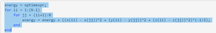
The objective function is the potential energy of the system, which is a sum over each electron pair of the inverse of their distances:
Define the objective function as an optimization expression.
energy = optimexpr;
for ii = 1:(N-1)
    for jj = (ii+1):N
        energy = energy + ((x(ii) - x(jj))^2 + (y(ii) - y(jj))^2 + (z(ii) - z(jj))^2)^(-1/2);
    end
end
elecprob.Objective = energy;
Start the optimization with the electrons distributed randomly on a sphere of radius 1/2 centered at [0,0,–1].
rng default % For reproducibility
x0 = randn(N,3);
for ii=1:N
    x0(ii,:) = x0(ii,:)/norm(x0(ii,:))/2;
    x0(ii,3) = x0(ii,3) - 1;
end
init.x = x0(:,1);
init.y = x0(:,2);
init.z = x0(:,3);
Solve the problem by calling solve. Time the solution.
tic
[sol,fval,exitflag,output] = solve(elecprob,init)
Solving problem using fmincon.

Local minimum found that satisfies the constraints.

Optimization completed because the objective function is non-decreasing in
feasible directions, to within the value of the optimality tolerance,
and constraints are satisfied to within the value of the constraint tolerance.

<stopping criteria details>
sol = struct with fields:
    x: [20×1 double]
    y: [20×1 double]
    z: [20×1 double]
fval =
163.0099
exitflag =
    OptimalSolution
output = struct with fields:
              iterations: 94
               funcCount: 150
         constrviolation: 0
                stepsize: 2.8395e-05
               algorithm: 'interior-point'
           firstorderopt: 8.1308e-06
            cgiterations: 0
                 message: 'Local minimum found that satisfies the constraints.↵↵Optimization completed because the objective function is non-decreasing in ↵feasible directions, to within the value of the optimality tolerance,↵and constraints are satisfied to within the value of the constraint tolerance.↵↵<stopping criteria details>↵↵Optimization completed: The relative first-order optimality measure, 8.090884e-07,↵is less than options.OptimalityTolerance = 1.000000e-06, and the relative maximum constraint↵violation, 0.000000e+00, is less than options.ConstraintTolerance = 1.000000e-06.'
            bestfeasible: [1×1 struct]
     objectivederivative: "reverse-AD"
    constraintderivative: "closed-form"
                  solver: 'fmincon'
toc
Elapsed time is 13.005444 seconds.
The solution time is over 10 seconds (your results might vary).
Modify Problem for Efficient Static Analysis
This video demonstrates the steps.
To make the optimization expression work more efficiently, extract the for loop and convert it to a local function. First, select the lines of code from energy = optimexpr; to the final end. Then, right-click the selected lines of code and choose Convert to Local Function.

Edit the resulting function (which appears at the end of this example) as follows:
Change the function name to
myenergy.Edit the first line of code to read:
energy = function myenergy(N, x, y, z);
In the second line of code, change the initial value from
optimexprto 0.
To take advantage of static analysis, place the energy into the problem as the objective function by calling fcn2optimexpr.
energy = fcn2optimexpr(@myenergy,N,x,y,z);
elecprob.Objective = energy;
Solve the problem by calling solve. Time the solution.
tic
[sol,fval,exitflag,output] = solve(elecprob,init)
Solving problem using fmincon.

Local minimum found that satisfies the constraints.

Optimization completed because the objective function is non-decreasing in
feasible directions, to within the value of the optimality tolerance,
and constraints are satisfied to within the value of the constraint tolerance.

<stopping criteria details>
sol = struct with fields:
    x: [20×1 double]
    y: [20×1 double]
    z: [20×1 double]
fval =
163.0099
exitflag =
    OptimalSolution
output = struct with fields:
              iterations: 94
               funcCount: 150
         constrviolation: 0
                stepsize: 2.8395e-05
               algorithm: 'interior-point'
           firstorderopt: 8.1308e-06
            cgiterations: 0
                 message: 'Local minimum found that satisfies the constraints.↵↵Optimization completed because the objective function is non-decreasing in ↵feasible directions, to within the value of the optimality tolerance,↵and constraints are satisfied to within the value of the constraint tolerance.↵↵<stopping criteria details>↵↵Optimization completed: The relative first-order optimality measure, 8.090884e-07,↵is less than options.OptimalityTolerance = 1.000000e-06, and the relative maximum constraint↵violation, 0.000000e+00, is less than options.ConstraintTolerance = 1.000000e-06.'
            bestfeasible: [1×1 struct]
     objectivederivative: "reverse-AD"
    constraintderivative: "closed-form"
                  solver: 'fmincon'
toc
Elapsed time is 0.630878 seconds.
The solution time decreases considerably, to under one second.
Compare with No Analysis
You can also solve the problem by treating the objective function as a black box. A black box objective cannot take advantage of automatic differentiation, so the solver must take finite difference steps to estimate the objective gradient. However, a black box can run quickly when the underlying function is fast to evaluate. Compare the solution time when you set fcn2optimexpr to create a black box objective.
energy = fcn2optimexpr(@myenergy,N,x,y,z,Analysis="off");
elecprob.Objective = energy;
tic
[sol,fval] = solve(elecprob,init)
Solving problem using fmincon. Solver stopped prematurely. fmincon stopped because it exceeded the function evaluation limit, options.MaxFunctionEvaluations = 3.000000e+03.
sol = struct with fields:
    x: [20×1 double]
    y: [20×1 double]
    z: [20×1 double]
fval =
163.3769
toc
Elapsed time is 0.381280 seconds.
The solver does not complete the optimization because it exceeds the function evaluation limit. Also, the resulting fval is higher than in the previous two solutions. Increase the function evaluation limit and try again.
opts = optimoptions("fmincon",MaxFunctionEvaluations=1e4);
tic
[sol,fval,exitflag,output] = solve(elecprob,init,Options=opts)
Solving problem using fmincon. Local minimum found that satisfies the constraints. Optimization completed because the objective function is non-decreasing in feasible directions, to within the value of the optimality tolerance, and constraints are satisfied to within the value of the constraint tolerance. <stopping criteria details>
sol = struct with fields:
    x: [20×1 double]
    y: [20×1 double]
    z: [20×1 double]
fval =
163.0099
exitflag =
    OptimalSolution
output = struct with fields:
              iterations: 97
               funcCount: 6039
         constrviolation: 0
                stepsize: 1.9714e-06
               algorithm: 'interior-point'
           firstorderopt: 5.5073e-06
            cgiterations: 0
                 message: 'Local minimum found that satisfies the constraints.↵↵Optimization completed because the objective function is non-decreasing in ↵feasible directions, to within the value of the optimality tolerance,↵and constraints are satisfied to within the value of the constraint tolerance.↵↵<stopping criteria details>↵↵Optimization completed: The relative first-order optimality measure, 5.480310e-07,↵is less than options.OptimalityTolerance = 1.000000e-06, and the relative maximum constraint↵violation, 0.000000e+00, is less than options.ConstraintTolerance = 1.000000e-06.'
            bestfeasible: [1×1 struct]
     objectivederivative: "finite-differences"
    constraintderivative: "closed-form"
                  solver: 'fmincon'
toc
Elapsed time is 0.645411 seconds.
The solution time is approximately the same as with static analysis, as is the objective function value. The output structure shows that the solver takes finite difference steps to estimate the objective gradient. The solver takes thousands of function evaluations, instead of fewer than 200 for the previous cases. If your function is time consuming to evaluate, this method might be inefficient.
Conclusions
Sometimes, you can save solution time by converting a for loop for static analysis. Converting a for loop to a function is fairly simple: highlight the loop, right-click to display the context menu, select the option for creating a local function or function file, and make minor edits to the new function.
In any case, use fcn2optimexpr to place your for loop expressions into your problem. This practice allows you to obtain any future improvements in static analysis automatically, without rewriting code.
Helper Function
The following code creates the myenergy helper function.
function energy = myenergy(N, x, y, z)
energy = 0;
for ii = 1:(N-1)
    for jj = (ii+1):N
        energy = energy + ((x(ii) - x(jj))^2 + (y(ii) - y(jj))^2 + (z(ii) - z(jj))^2)^(-1/2);
    end
end
end