Create Route Planner for Offroad Navigation Using Digital Elevation Data

Since R2024a

Step 1 of 5 in Offroad Navigation for Autonomous Haul Trucks in Open Pit Mine

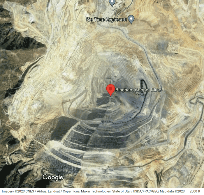
This example shows how to approximate a road network using point cloud terrain data representing an open-pit mine. The point cloud data, composed of multiple LAZ files merged together, is from the U.S. Geological Survey database and represents a copper mine in Bingham Canyon, Utah. Locations like this copper mine present a mix of structured and unstructured terrain, indicating that might need different planning techniques based on the characteristics of the terrain and the application.

This image shows the formation of switchbacks leading into the mine. While Google Maps™ lacks road-network data for the interior of the mine, you can use the terrain data to reconstruct the structural layout.

Extract Elevation Data from Point Cloud

Download the cleanedUSGSPointCloud.zip file from the MathWorks® website, unzip the file, and then load the point cloud. The point cloud is approximately 38 MB and produced by the United States Geological Survey using an aerial lidar sensor [1].

data = matlab.internal.examples.downloadSupportFile("nav","data/pitMineClean.mat");
load(data,"cleanPC")

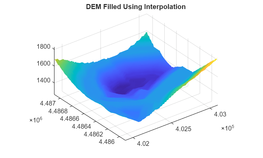
Convert the raw point cloud to a digital elevation model (DEM) using the exampleHelperPc2Grad helper function. This helper function first uses the pc2dem function to sample the initial elevation over the xy-limits of the point cloud. Then, it fills in missing regions of the elevation matrix using the scatteredInterpolant function. Lastly, it computes the gradient using the griddedInterpolant function.

res = 1; % Resolution of 1 cell per meter
[dzdx,dzdy,dem,xlims,ylims,xx,yy] = exampleHelperPc2Grad(cleanPC,res);

Visualize the original point cloud data.

figure
pcshow(cleanPC)
title("USGS Point Cloud")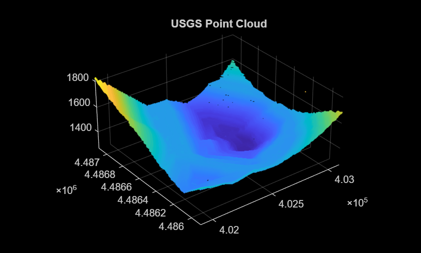

Next, show the surface with gaps filled using interpolation.

figure
hSurf = surf(xx,yy,dem,EdgeColor="none");
title("DEM Filled Using Interpolation")
axis equal

Construct Road Network

Identify Road Boundaries

With the slope information from the DEM, you can identify the boundaries of the traversable regions to create a road network. Note that slope is just one way you can draw out structure from data representing an environment. Other methods include semantic segmentation of an aerial image, or generating obstacle boundaries using sensor data.

Set the maximum slope that the haul truck can traverse to 15 degrees.

slopeMax = deg2rad(15);

Create a gradient mask to identify the traversable regions using the maximum slope threshold.

maskSlopeX = atan2(abs(dzdx),1/res) < slopeMax;
maskSlopeY = atan2(abs(dzdy),1/res) < slopeMax;
imSlope = maskSlopeX & maskSlopeY;

Display off-limit areas where the slope is greater than the maximum slope threshold. Using this gradient mask, you can see the road switchbacks.

figure
imshow(imSlope)
title("Traversable Regions in Pit Mine")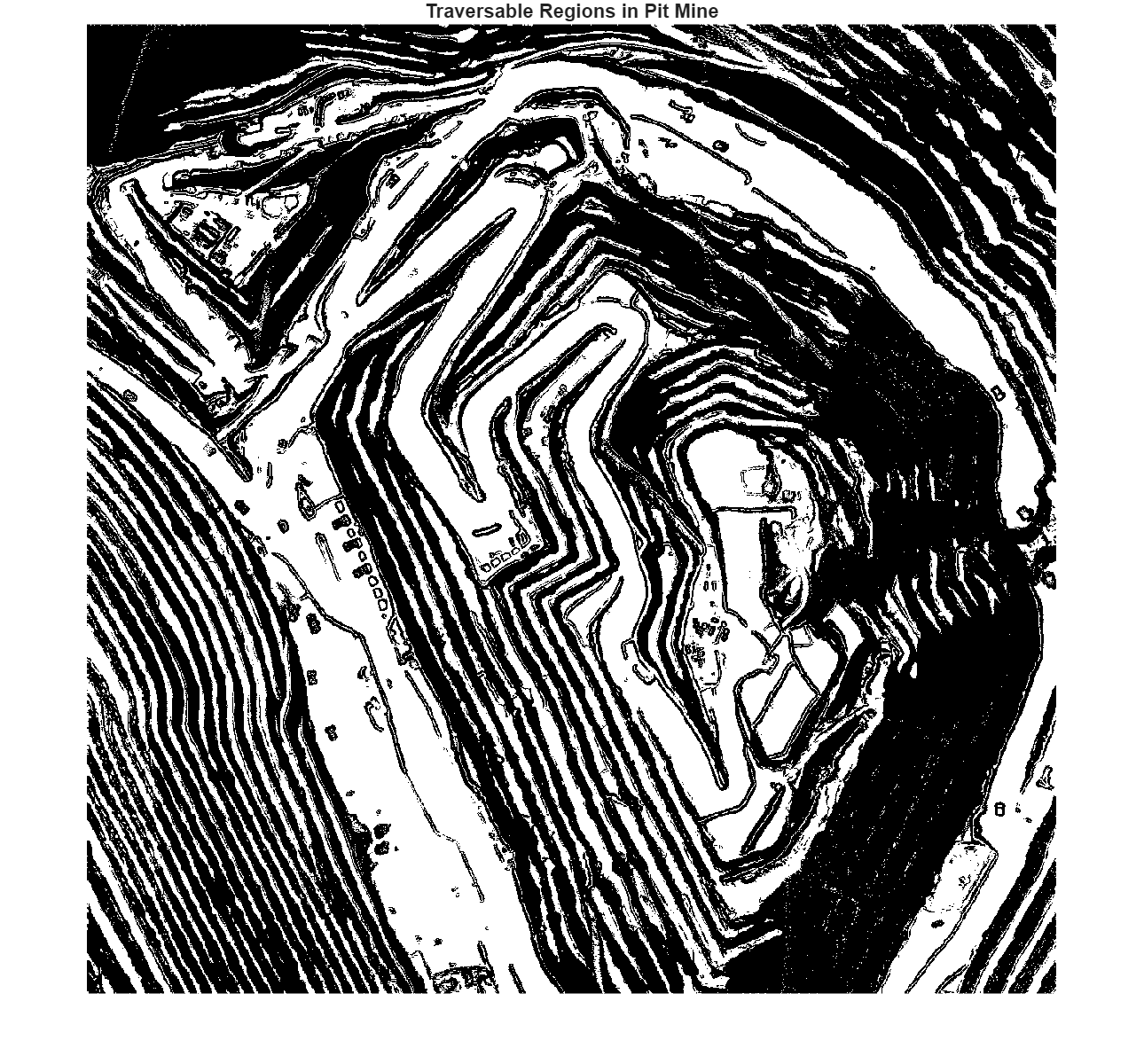

Clean DEM Gradient Mask

To perform accurate path planning through the pit mine, you must ensure that the gradient mask contains minimal noise. Although you can use the raw gradient mask for path planning, any noise it contains can result in disconnected edges or an excessive number of paths through confined spaces. To produce a more practical road network, you can apply several morphological operations to the gradient mask.

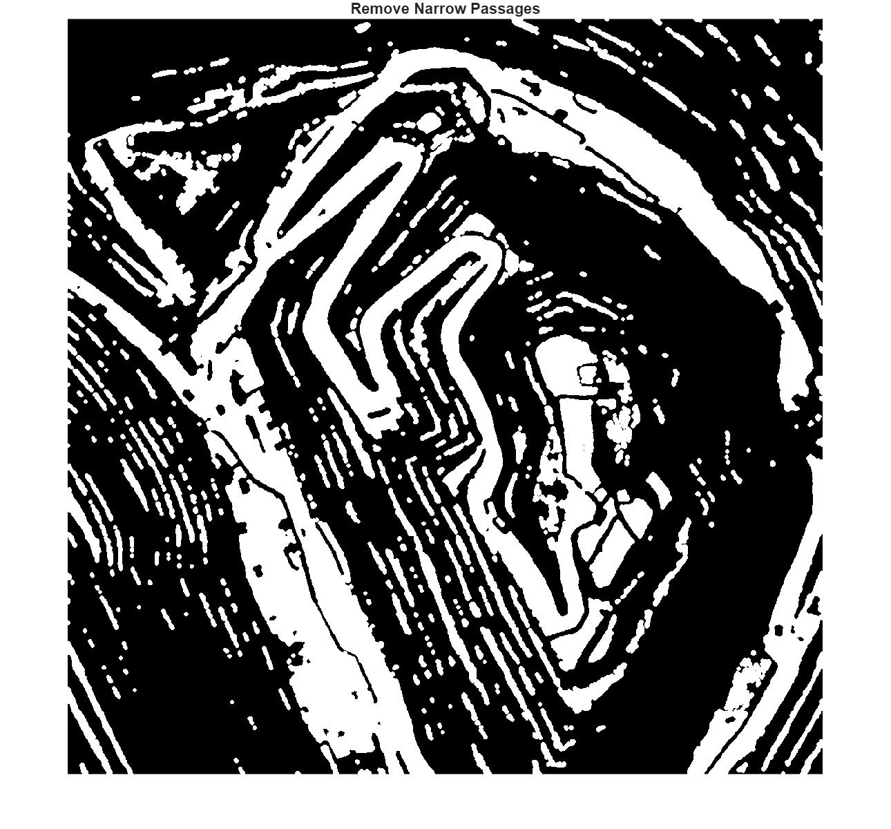
First, use the imopen (Image Processing Toolbox) function to fill in small gaps within the maximum slope regions to produce more consistent road boundaries and filter out narrow passages.

se = strel("disk",4);
imNarrow = imopen(imSlope,se);
imshow(imNarrow)
title("Remove Narrow Passages")

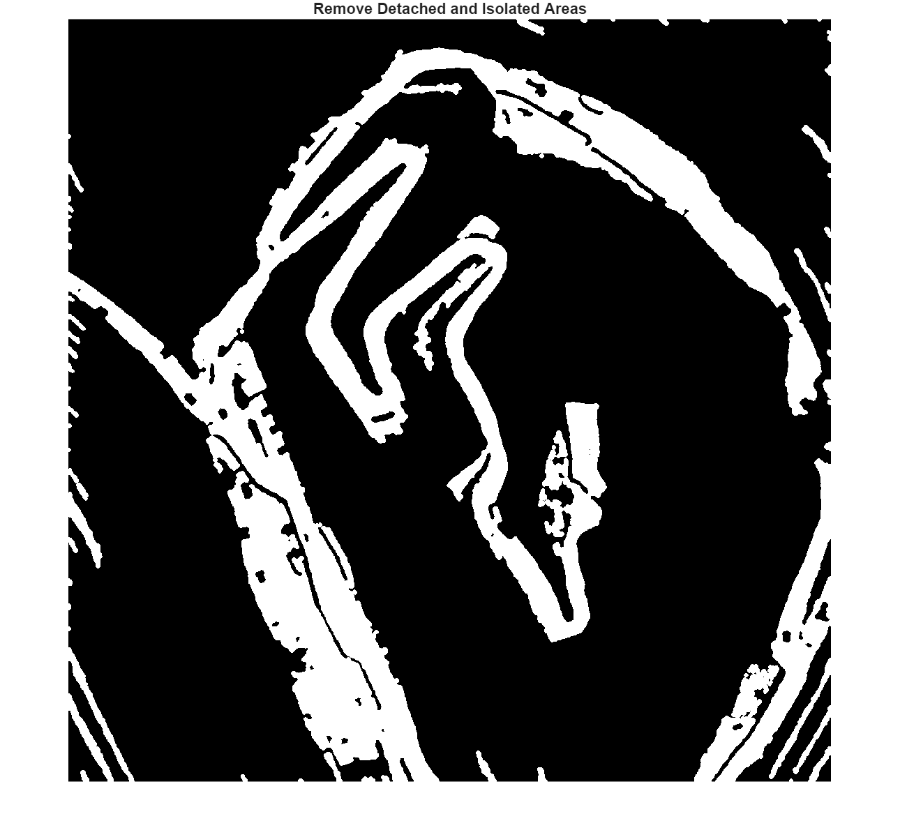
Next, use the imfill (Image Processing Toolbox) function to remove small, isolated areas that are detached from the main traversable sections of the map. Since you cannot reach these areas from the road network, they are irrelevant during route planning.

imHoles = ~imfill(~imNarrow,"holes");
imshow(imHoles)
title("Remove Detached and Isolated Areas")

Use the bwboundaries (Image Processing Toolbox) function to remove small areas that have an above-average slope. This change ensures that roads go straight through the open areas, rather than splitting into multiple paths to bypass small bumps or uneven spots in the ground.

% Identify any holes that might remain
[B,~,~,~] = bwboundaries(imHoles);
[val,idx] = sort(cellfun(@(x)size(x,1),B));

% Remove interior occupied regions with small boundaries
i = 1;
seedPts = zeros(0,2);
perimeterSizeThreshold = 20; % in cells
while (val(i) < perimeterSizeThreshold)
    ij = B{idx(i)};
    seedPts = [seedPts; ij(1,:)]; %#ok<AGROW>
    i = i + 1;
end

Lastly, use the imdilate (Image Processing Toolbox) function to reinforce and clearly define any remaining boundaries.

pixelConnectivity = 4;
diskRadius = 3;
imFilled = ~imdilate(bwmorph(~imfill(imHoles,seedPts,pixelConnectivity),"bridge"),ones(diskRadius));
imshow(imFilled)
title("Reinforce Boundaries and Remove Small Road Bumps")

Convert Cleaned Gradient Mask Image into Skeleton

After refining the gradient mask, skeletonize the image using the bwskel (Image Processing Toolbox) function. This process transforms all traversable areas in the gradient mask into one-pixel-wide roads, effectively reducing the roads into their most basic structural form.

rawSkel = bwskel(imFilled,MinBranchLength=75);
se = strel(disk=3);

Show the skeleton of the gradient mask.

f2 = figure;
imshow(rawSkel)
title("Raw Skeleton")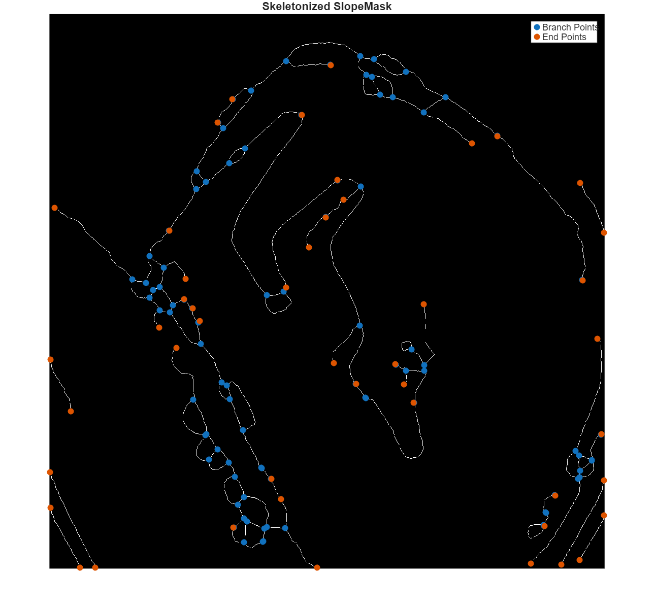

hAx = f2.CurrentAxes;

Now you have a network of traversable paths, but it lacks connectivity information.

Use the bwmorph function to identify branch points, where the path splits into two or more paths.

branchPts = bwmorph(rawSkel,"branchpoints");

Use bwmorph again to identify the end points of the paths.

endPts = bwmorph(rawSkel,"endpoints");
[val,idx] = sort(cellfun(@(x)size(x,1),B));

Display both the branch points and end points on top of the skeleton.

[ib,jb] = ind2sub(size(branchPts),find(branchPts'));
[ie,je] = ind2sub(size(branchPts),find(endPts'));
hold on
scatter(hAx,ib(:),jb(:),"o","filled")
scatter(hAx,ie(:),je(:),"o","filled")

title(hAx,"Skeletonized SlopeMask")
legend(hAx,{"Branch Points","End Points"})
hold off

Extract Edges from Skeleton

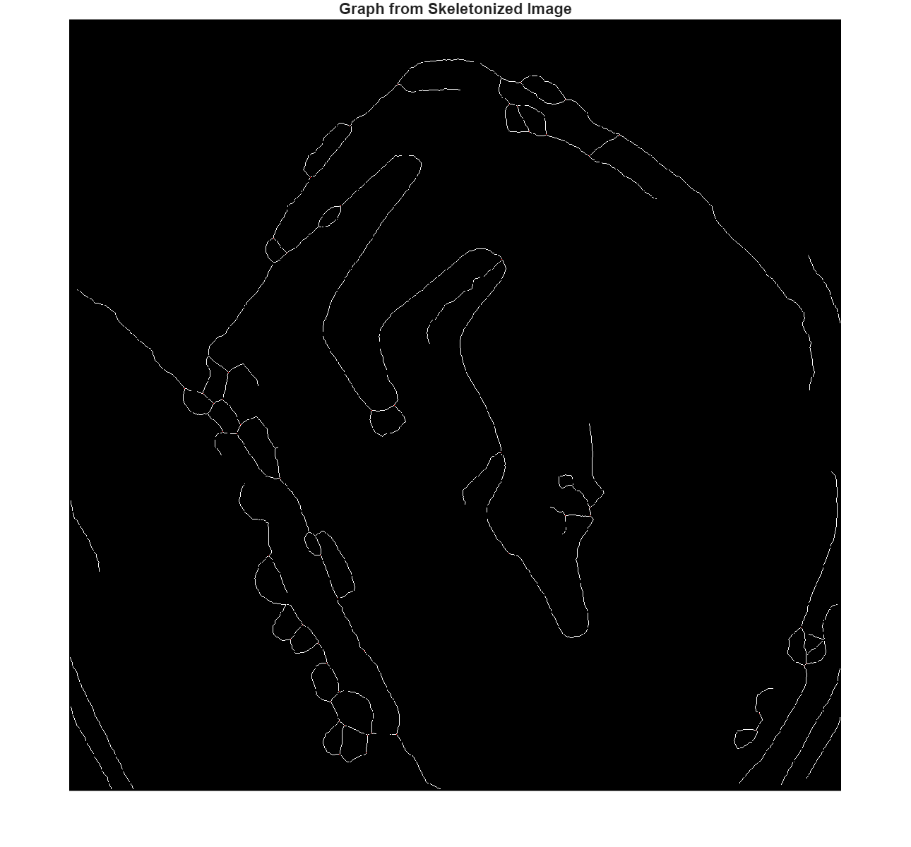
While you can start path planning using the skeleton, you can further improve your path-planning efficiency by breaking the skeleton up into branches. The exampleHelperSkel2Edges helper function does this by starting at each end point and visiting the next free neighbor until it finds another end point or branch point. The helper function also applies this process to pathways stemming from branching points. Throughout this process, the function documents each cell that it traverses along each edge in a respective element of a structure array, enabling a structured representation of the individual network paths.

Use the exampleHelperSkel2Edges helper function to build the list of paths and visualize the graph from the skeletonized image.

figure
[pathList,cleanSkel] = exampleHelperSkel2Edges(rawSkel,Visualize=true);

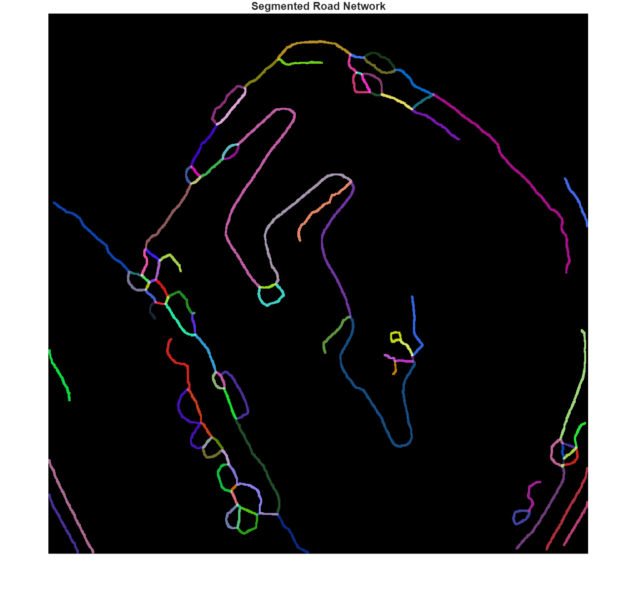
Visualize the set of unique road segments derived from the terrain.

hImg = imshow(cleanSkel);
exampleHelperOverlayPathImage(hImg,pathList,rand(100,3),Radius=3,Frame="ij")
title("Segmented Road Network")
hold on

Convert Edges into Navigation Graph

The last step is to convert your set of edges into a navGraph object, which you can use return the shortest paths between any two nodes in the road network. The exampleHelperPath2GraphData helper function takes in the list of edges generated by the exampleHelperSkel2Edges helper function and converts it to a set of connected nodes and the edges that connect them.

First, create a binary occupancy map using the slope data, and then convert the grid coordinates to local xy-coordinates.

binMap = binaryOccupancyMap(~imSlope,1);
localPathList = pathList;
for i = 1:numel(pathList)
    localPathList(i).Path = grid2local(binMap,pathList(i).Path);
end

Use the exampleHelperPath2GraphData helper function to convert the raw path list into graph information.

[nodes,edges,edge2pathIdx,cachedPaths] = exampleHelperPath2GraphData(localPathList);

When developing a route-planner, you must consider the density of the graph, which is the level of detail or granularity in representing possible paths. The exampleHelperPath2GraphData helper function addresses this by accepting an optional argument, edgeSize, that controls how frequently to subdivide the edges when converting the path list to a graph. When edgeSize is the default value of inf, the graph construction relies solely on endpoints, resulting in a compact and computationally efficient search space. This approach enables a balance between detail and performance, ensuring that the route-planning process remains both accurate and manageable.

maxEdgeSize = 25;
[denseNodes,denseEdges,denseEdge2pathIdx,denseCachedPaths] = exampleHelperPath2GraphData(localPathList,maxEdgeSize);

Display the number of edges and the number of dense edges. Note that the number of edges has increased due to the maxEdgeSize argument.

disp(size(edges,1))

   226

disp(size(denseEdges,1))

   832

A navGraph object also enables you to use custom edge costs to consider qualities like path length, elevation, slope, or even dynamic congestion for multiple-agent path planning. In this case, compute the accumulated lengths along the dense path edges to use as the costs associated with each edge.

edgeCosts = exampleHelperDefaultEdgeCost(denseCachedPaths,denseEdge2pathIdx);

Store additional metadata about the edges of the graph.

Create a state table that stores the nodes with their corresponding states. Next, create a link table, which stores the edges, their respective costs, and the Edge2PathIdx mapping. In this route planner, Edge2PathIdx serves as a link between the edges of the graph and the comprehensive set of dense paths stored in cachedPath. This enables you to fully reconstruct the path between any two nodes after planning a route.

stateTable = table(denseNodes,VariableNames="StateVector");
linkTable = table(denseEdges,edgeCosts,denseEdge2pathIdx(:), ...
    VariableNames=["EndStates","Weight","Edge2PathIdx"]);

Create the navGraph object using the state and link tables.

sparseGraph = navGraph(stateTable,linkTable);

Find Shortest Path Using A*-Based Route Planner

Create the A* path planner using the navGraph.

planner = plannerAStar(sparseGraph);

Define a start location and a goal location.

start = [286.5 423.5];
goal  = [795.5 430.5];

Find the relative positions of each node in the start and goal locations. Then find the nodes with the shortest distance to the start and goal locations.

relPosStart = denseNodes(:,1:2)-start(1:2);
relPosGoal = denseNodes(:,1:2)-goal(1:2);
[dStart,nearStartIdx] = min(vecnorm(relPosStart,2,2));
[dGoal,nearGoalIdx] = min(vecnorm(relPosGoal,2,2));

Plan a route using just the graph.

[waypoints,solnInfo] = plan(planner,nearStartIdx,nearGoalIdx);

The planning process utilizes a sparse graph to quickly plan paths, but this planned path is a simplified representation.

To reconstruct the full path, first get the edge pairs from the solution info and the link IDs for those edge pairs. Then, get the full path using the Edge2PathIdx column of the link table and the link IDs.

edgePairs = [solnInfo.PathStateIDs(1:end-1)' solnInfo.PathStateIDs(2:end)'];
linkID = findlink(planner.Graph,edgePairs);
networkPath = vertcat(denseCachedPaths(planner.Graph.Links.Edge2PathIdx(linkID)).Path);

Visualize Planned Path

Visualize the full road network.

figure
hIm = show(binMap);
cmap = colormap("spring");
exampleHelperOverlayPathImage(hIm,pathList,cmap(randi(size(cmap,1),100),:),Radius=2)
title("Full Road Network")
hold on

Plot the edge nodes of the graph on top of the road network.

gHandle = show(planner.Graph);
gHandle.XData = planner.Graph.States.StateVector(:,1); 
gHandle.YData = planner.Graph.States.StateVector(:,2);
gHandle.MarkerSize = 2;
gHandle.LineWidth = 1.25;
gHandle.ShowArrows = "off";
gHandle.NodeLabel = {}; % Remove node labels to reduce clutter
title("Path Edge Nodes")

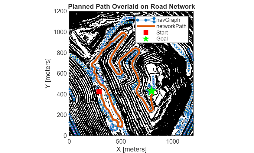
Lastly, overlay the planned path on the road network.

exampleHelperPlotLines(networkPath,{"LineWidth",3})

ans = 
165.0021

startSpec = plannerLineSpec.start(MarkerEdgeColor="red",MarkerFaceColor="red");
goalSpec = plannerLineSpec.goal(MarkerEdgeColor="green",MarkerFaceColor="green");
plot(start(1),start(2),startSpec{:})
plot(goal(1),goal(2),goalSpec{:})
title("Planned Path Overlaid on Road Network")
legendStrings = ["navGraph","networkPath","Start","Goal"];
legend(legendStrings)
hold off

Conclusion

In this example, you learned to extract structural information from USGS-sourced terrain data to develop a route planner. The process starts with extracting the gradient from a digital elevation model. Next, you apply morphological operations to a slope-masked image to identify traversable areas. You then skeletonize the free space, with the resultant edges creating the boundaries of an implicit Voronoi field. Lastly, you convert this skeleton into a graph, which you can then use as a basic route planner.

In the next example, Create Onramp and Terrain-Aware Global Planners for Offroad Navigation example, in which you develop two planners. The first is an onramp planner that can generate paths to get onto the graph while complying with the non-holonomic constraints of a haul truck, and the second is a terrain-aware planner for navigating unstructured regions of the pit mine using plannerHybridAStar.

References

1. cleanPC compiled from National Map 3DEP Downloadable Data Collection courtesy of the U.S. Geological Survey.