SystemVerilog Module Generation
This example shows how to export the ADC subsystems individually as C code encapsulated with a direct programming interface (DPI) wrapper and import them as SystemVerilog modules in a mixed-signal simulation. This enables you to quickly instantiate a reference design including impairments or generate a complex testbench for your mixed-signal simulation.
This part of the tutorial is based on the model:
model = 'MSADCTutorial_dpic.slx';
open_system(model);
The following are the steps you need to take to export the model.
Use the fixed step solver
Specify the C code generation target
Generate SystemVerilog modules for each subsystem
Create a testbench in Cadence Virtuoso AMS Designer
Write a SystemVerilog scheduler
Set up the model for execution
The reference Cadence library can be found in the archive ADC_DPI.tar.gz in this location.
location = [matlabshared.supportpkg.getSupportPackageRoot '/toolbox/msblks/supportpackages/msblksmodels/mdllibs/ADC'];
cd(location);
Use the Fixed-Step Solver
The first and most critical step is to use a fixed step solver, as the generated C code needs to have a fixed notion of time to operate on and update its internal states. You must choose the fixed step size greater than the sampling rate or frequency of the internal signals, to capture the block functionality while minimizing the error introduced when changing the solver configuration. To change the solver, open the model configuration parameter and change type in the solver tab.
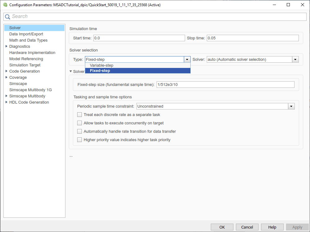
At this step, you can either enter the fixed-step size manually or use the default auto option that automatically inherits the period of the fastest sampling rate. You can re-run the simulation and compare the results with two solver configurations. In order to verify the consistency of the results you must compare the difference in the output against the original simulation and define a maximum tolerance. As the antialiasing filter is defined in Simscape Electronics using an electrical network, it is important to choose the right step size to translate the model execution from continuous-time to discrete-time.
In this case, the fastest data rate in the model is 512 kHz (output of the ADC) and you can choose e.g., a time step equal to 1/512e3/10 = 1.9531e-07.
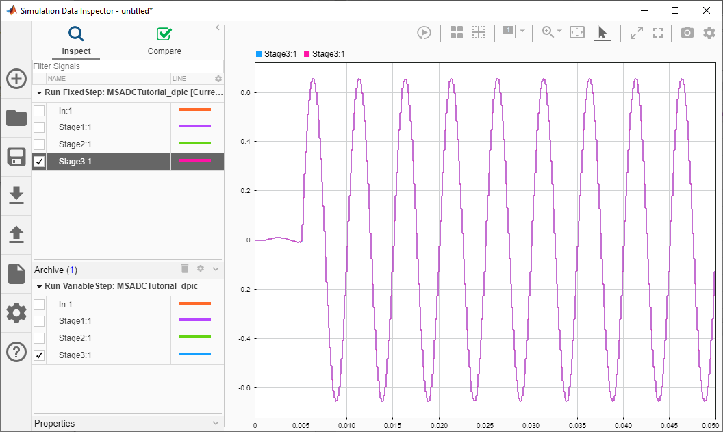
For comparing the results you can use the Simulation Data Inspector.

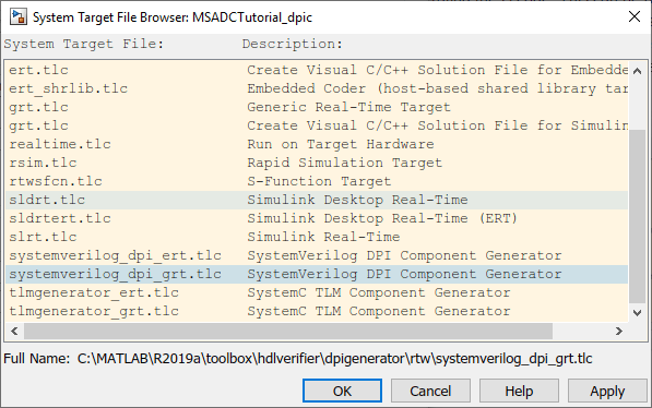
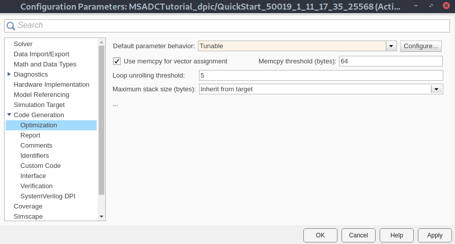
Specify the C Code Generation Target
The second step is to specify the target for generating C code. This can be done by navigating to Code Generation tab on the model configuration parameters window opened in the first step. You choose SystemVerilog DPI Component Generator as the System Target File. You can choose the target for a generic real time (GRT) target or embedded real time (ERT) target. The latter option provides more alternatives for c-code optimization and customization.
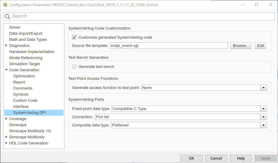
After selecting the target file, you need to customize the wrapper to be pin-compatible with the Simulink subsystem. The custom wrapper avoids having additional input signals such as clock and enable. Although these signals can be useful in a digital context, they are not required for this specific application.
Generate SystemVerilog Modules for Each Subsystem
You now select the blocks to be exported, and right click, select 'C/C++ Code>Build This Subsystem'. The C code for each of these blocks is put in a separate folder in the current directory along with the makefile (.mk), DPI wrapper and SystemVerilog module (.sv), and all the header files required to compile the code.
You repeat this operation for each of the subsystems: Sine Source, Circuit-Level Analog Filter, Delta-Sigma Order II, and Decimator.
Click on "Configure" from the Optimization tab under Code Generaration to configure the tunable parameters. The Sine Source block specifies two tunable parameters: A, representing the amplitude of the sinusoidal excitation, and F, representing its frequency. You define the two parameters to use "ExportedGlobal" storage class. This makes sure that A and F will be tunable parameters also in the generated SystemVerilog module.
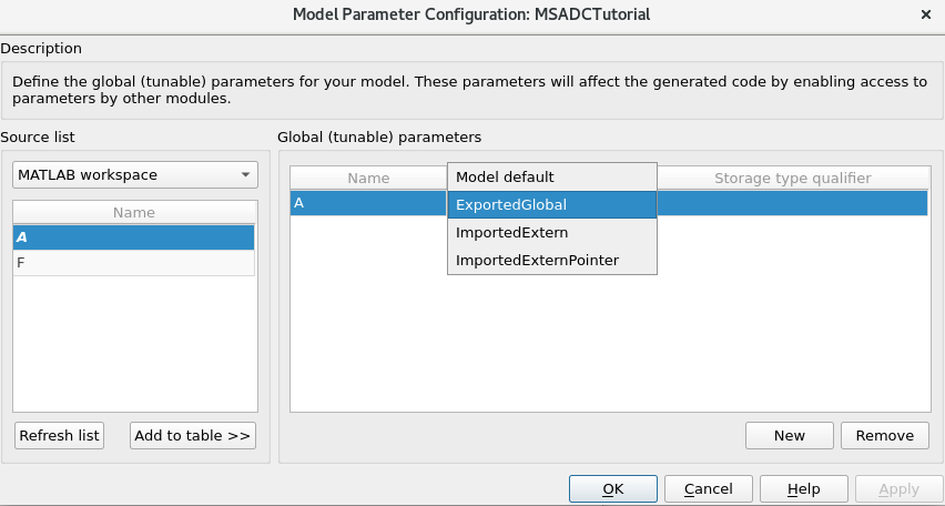
Other blocks do not specify tunable parameters. At the end of the code generation process, you get a dedicated folder for each subsystem including all the required files. The files need to be compiled to create one shared library (so on Linux®) for each of the subsystems.
Verify the Design Using Cadence Incisive
You can use the DPI-C models to verify the design in Cadence environment.
Create a Testbench in Cadence Virtuoso AMS Designer
You need to create a new cellview for each block in the AMS Designer. For module definition you can either link or copy the DPI-C wrapper of each block with its cellview. It is preferable to create a symbolic link to the automatically generated SystemVerilog modules, as this will capture eventual modifications to the block interface.
Each of the generated blocks has a systemVerilog view and a symbol view. The testbench cellview is a schematic, requiring a config view for model elaboration.
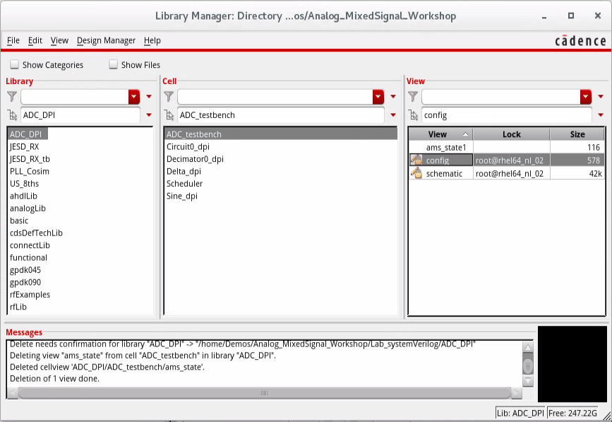
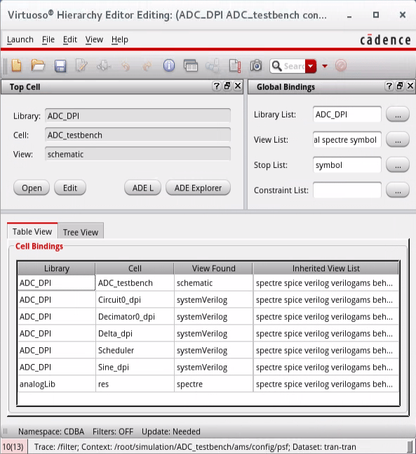
The first time you open a systemVerilog module in AMS Designer, a symbol is automatically created for block instantiation. The cellviews need to be instantiated in the testbench schematic one at a time and connected in the same sequence. The name of each block instance is important, as this will be referenced by the scheduler.
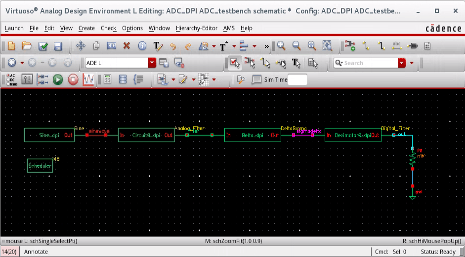
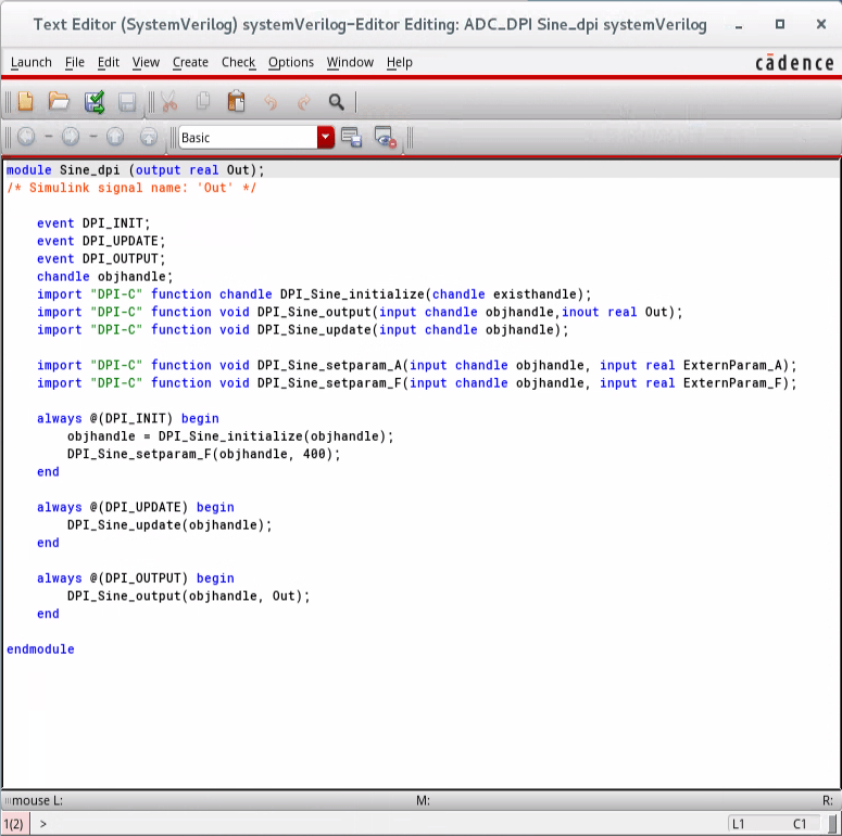
Write a SystemVerilog Scheduler
To run the simulation, you need a scheduler block to drive the execution order of the blocks in the testbench. The SystemVerilog module automatically generated for each block identifies 3 phases:
initialization: occurs at the start of the simulation
output: compute the output at each desired rate
update: update the internal states based on the input signals
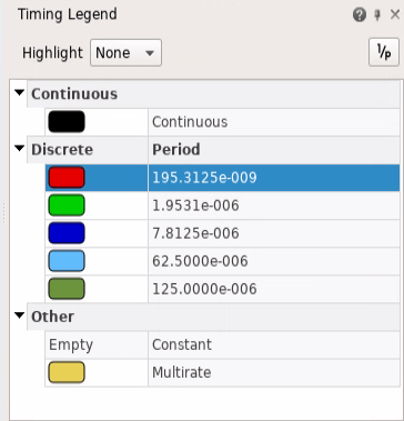
The SystemVerilog scheduler defines the sequence of execution of these three phases for each block. As the original Simulink model is multi-rate, you can recognize two major rates of execution.
The sinusoidal waveform, the analog filter, and the second order delta sigma converter operate at the fastest rate as defined by the fixed-step solver. In this case, the sample time is equal to 1/512e3/10 = 195.31 ns. As the scheduler uses a time scale defined in nanoseconds, we can approximate the fastest rate of execution with a clock with period equal to 200 ns.
The decimator block operates at a slower rate, equal to 1/512e3 = 1953 ns. In this case, you can approximate the rate of execution with a clock with a period of 2000 ns. You can improve the clock accuracy for example using a finer timescale.

To know what is the original execution rate in the Simulink model, you can use the sample time legend.
Set up the Model for Execution
To start the simulation, you must launch ADE-L, choose ams as the simulator and select a transient analysis. Before launching the simulation, you must also link and load the shared objects created for each block.
From ADE-L, open Simulation>Options>AMS simulator options.
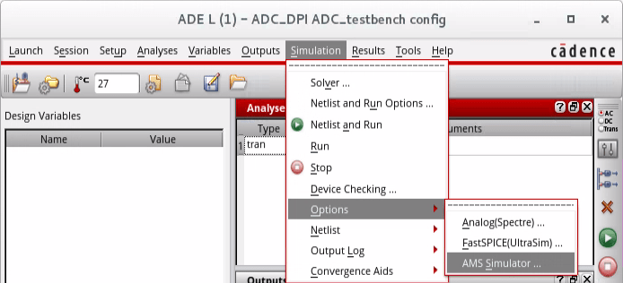
From the AMS options menu, open the additional arguments pane and list with the -sv_lib option for all the shared libraries.
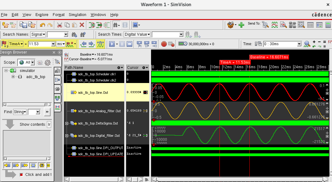
You can launch the simulation and verify the function of each block in the mixed-signal simulation environment. The following figure shows the simulation results of a 30s transient simulation of the model. The outputs of all the blocks are consistent with Simulink simulation. Small differences are due to the different timescale used by the scheduler.
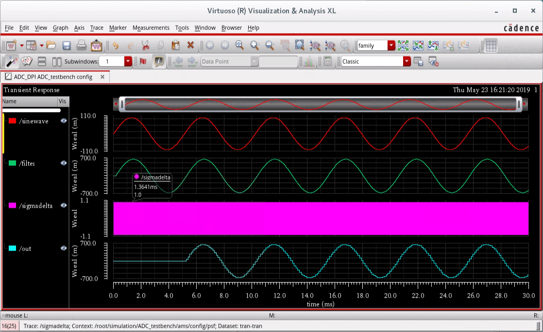
You can also, for example, change the frequency of the sinusoidal excitation in the source block. In the SystemVerilog module of the source, for example at initialization you can change the frequency to 400 Hz instead of the default 200 Hz.
Verify the Design Using Cadence Xcelium
If you do not have access to Cadence Virtuoso for verifying your design using Incisive, you can use Cadence Xcelium to verify your design. You will use the same model that is used in the introduction.
model='MSADCTutorial_dpic';
open(model);
Generate DPI-C Models
Run the following commands to generate DPI-C models for each subsystem in the model.
cfg = getActiveConfigSet(model);

%Pick Target file for DPI-C gen
switchTarget(cfg,'systemverilog_dpi_grt.tlc',[]);
cfg.set_param('DPICustomizeSystemVerilogCode', 'on');   % Customize generated SystemVerilog code
cfg.set_param('GenerateReport', 'off');   % Dont Create code generation report
cd('work');

% Build SV DPI-C models
slbuild([model, '/SineSource']);
slbuild([model, '/AnalogFilter']);
slbuild([model, '/DeltaSigma']);
slbuild([model, '/Decimator']);
All the DPI build folders are generated in the directory called work. Also the RTL generated by HDL coder for the Decimator can be found under work/hdlsrc directory. For instructions on how to generate HDL Code for the Decimator, see System-Level Model of DSM ADC.
Run Simulation
To run the simulation using Xcelium, from Linux C shell, under work/tb_top folder, review the shell script "runsim.sh". To simulate with the SV DPIC model of Decimator, launch the shell script from your C shell as shown below.
sh runsim.sh
To simulate with the RTL of Decimator, launch the shell script from your C shell as shown below.
sh runsim.sh RTL
If you encounter the following error when you run the simulations, check that the modules names in tb_top/run.f and tb_top/adc_tb_top.sv match the folder names generated by slbuild.
xrun: *E,FILEMIS: Cannot find the provided file
Either of the above two commands will launch the simulation using Xcelium digital solver. The ADC waveforms will be visible on SimVision after the completion of simulation.
Summary: Digital Filter Design
You have converted to fixed-point the digital decimation filter, and explored a workflow suitable for fractional length optimization. For the multi-rate multi-stage filter you have generated synthesizable HDL code and validated the results using cosimulation with Cadence Incisive. You have also reviewed how to validate your design using Cadence Xcelium.
You can now proceed to the final section of this tutorial, Final System-Level Model.