Choose Extrapolation Method Based on Application
This example shows how to choose the right extrapolation method based on your design. It also shows how to use extrapolation method to predict the values eye metrics at symbol error rates beyond those captured in an eye diagram. You can see the strengths and weaknesses of each extrapolation or interpolation method.
Find Eye Width of PAM2 Signal
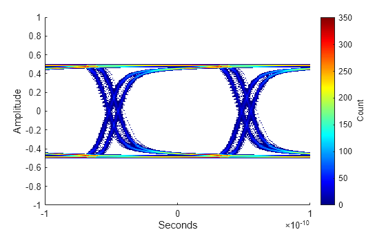
Load a PAM2 waveform with low noise, a fast slew rate relative to its unit interval, and jitter consisting of a significant duty cycle distortion (DCD) and a normally distributed random jitter (RJ) component. Load two eye diagrams derived from the waveform: one made from 2000 symbols and the other made from 20 million symbols.
load("extrapolate_pam2.mat", "ed2k", "ed20M");
plot(ed2k);
The original data contained approximately 2000 samples, which means the smallest measured symbol error rate (SER) should be around 1 / 1000. But some applications require eye metrics at much smaller SER values, such as 1e-7, which is what this example uses.
ser = 1e-7;
You can use any of the available two extrapolation methods and five interpolation methods to predict the size of the eye opening for a longer dataset, based on the measurement of the current dataset. Compare each against a long simulation, using bathtub curves.
Available Extrapolation Methods
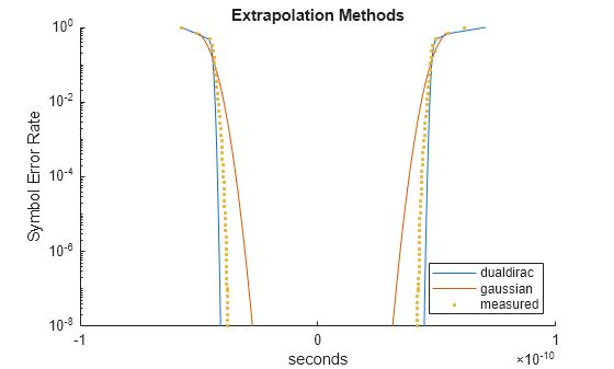
dualdirac- This method performs a curve fit of the Dual-Dirac jitter model's PDF to a slice of the eye diagram, then uses the coefficients of that fitted model to solve the corresponding quantile for the specified symbol error rate to find the position of the eye contour.gaussian- This method uses the sample mean and sample standard deviation of a slice of the eye diagram to define a Gaussian curve. It then solves the Gaussian quantile for the specified symbol error rate to find the position of the eye contour.
bathtub(ed2k, "horizontal", 0, "Extrapolation", "dualdirac", "SER", ser);
hold on
bathtub(ed2k, "horizontal", 0, "Extrapolation", "gaussian", "SER", ser);
bathtub(ed20M, "horizontal", 0, "Extrapolation", "linear", "SER", ser, "Marker", ".", "LineStyle", "none");
hold off
title("Extrapolation Methods");
legend("dualdirac", "gaussian", "measured", "Location", "southeast");
Available Interpolation Methods
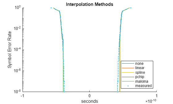
none- Previous neighbor interpolation of the cumulative sum of an eye slice, outward from the center of the eye.linear- Linear interpolation of the cumulative sum of an eye slice.spline- Natural spline interpolation of the cumulative sum of an eye slice.pchip- PCHIP interpolation of the cumulative sum of an eye slice.makima- Modified Akima interpolation of the cumulative sum of an eye slice.
bathtub(ed2k, "horizontal", 0, "Extrapolation", "none", "SER", ser);
hold on
bathtub(ed2k, "horizontal", 0, "Extrapolation", "linear", "SER", ser);
bathtub(ed2k, "horizontal", 0, "Extrapolation", "spline", "SER", ser);
bathtub(ed2k, "horizontal", 0, "Extrapolation", "pchip", "SER", ser);
bathtub(ed2k, "horizontal", 0, "Extrapolation", "makima", "SER", ser);
bathtub(ed20M, "horizontal", 0, "Extrapolation", "linear", "SER", ser, "Marker", ".", "LineStyle", "none");
hold off
title("Interpolation Methods");
legend("none", "linear", "spline", "pchip", "makima", "measured", "Location", "southeast");
The extrapolation methods provide a pessimistic estimate, while the interpolation methods provide an optimistic one. In this case, the application suits the Dual-Dirac model: we are finding a timing-based metric, eye width, the signal is PAM2, and the jitter is composed of a binary deterministic component and a normally-distributed random component.
eyeWidth(ed2k, 0, "Extrapolation", "dualdirac", "SER", ser, "Plot", "on")
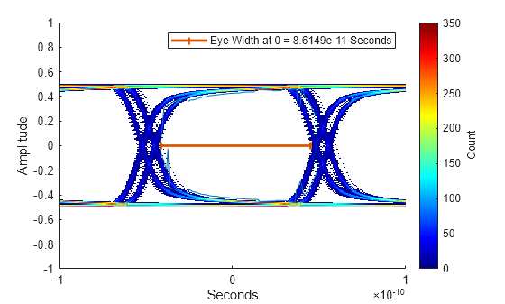
ans =
8.6149e-11
Find Eye Height Trend of PAM4 Signal
Load a set of PAM4 waveforms with intersymbol interference and thermal effects being the primary contributors to noise. The data represents a set of simulations of the same circuit, taken at different ambient temperature values. Each simulation ran for 1000 symbols. Load the cell array of eye diagrams and the corresponding vector of temperature values.
load("extrapolate_pam4.mat", "eyes", "temps");
Create a table to organize the temperatures and eye diagrams:
tbl = table(temps', eyes', 'VariableNames', ["Temperature", "EyeDiagram"])
tbl=11×2 table
    Temperature        EyeDiagram
    ___________    __________________

          0        {1×1 eyeDiagramSI}
         10        {1×1 eyeDiagramSI}
         20        {1×1 eyeDiagramSI}
         30        {1×1 eyeDiagramSI}
         40        {1×1 eyeDiagramSI}
         50        {1×1 eyeDiagramSI}
         60        {1×1 eyeDiagramSI}
         70        {1×1 eyeDiagramSI}
         80        {1×1 eyeDiagramSI}
         90        {1×1 eyeDiagramSI}
        100        {1×1 eyeDiagramSI}
Plot the eye diagrams, labeled with the corresponding temperature.
f = figure;
f.Position = [100, 100, 2148, 2148];
for i = 1:size(tbl, 1)
    nexttile;
    plot(tbl.EyeDiagram{i});
    title(tbl.Temperature(i) + " degrees Celsius");
end
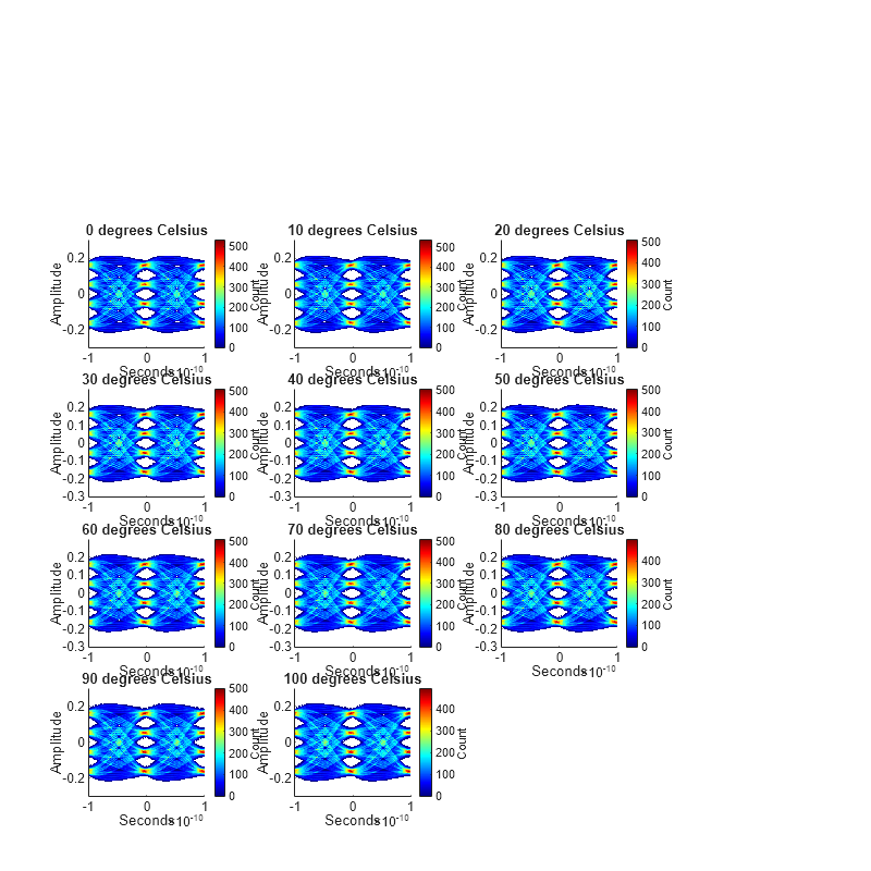
As you can see, there is little variation between individual eyes in this view. But you can use interpolation or extrapolation to characterize trends smaller than a bin in the measured data.
Of the available interpolation methods, none is not useful here, since it does not show the sub-bin differences that you want to see.
For extrapolation, the signal in question is PAM4 and the metric in question is height-related, and so it is not compatible with the assumptions of the Dual-Dirac jitter model.
First, find the trend in measured eye heights at a SER of 0.01 using linear interpolation. Then, find the trend in extrapolated eye heights at a SER of 1e-5 using gaussian extrapolation.
interpolatedHeight = zeros(size(tbl, 1), 3);
extrapolatedHeight = zeros(size(tbl, 1), 3);
for i = 1:size(tbl, 1)
    interpolatedHeight(i,:) = eyeHeight(tbl.EyeDiagram{i}, "Extrapolation", "linear", "SER", 0.01);
    extrapolatedHeight(i,:) = eyeHeight(tbl.EyeDiagram{i}, "Extrapolation", "gaussian", "SER", 1e-5);
end
Add the new vectors to the data table.
tbl.("Interpolated") = interpolatedHeight;
tbl.("Extrapolated") = extrapolatedHeight
tbl=11×4 table
    Temperature        EyeDiagram                  Interpolated                        Extrapolated
    ___________    __________________    ________________________________    ________________________________

          0        {1×1 eyeDiagramSI}    0.066393    0.066782    0.066858    0.030514    0.030808    0.030339
         10        {1×1 eyeDiagramSI}    0.066137    0.066601    0.066631    0.030421    0.030592    0.030141
         20        {1×1 eyeDiagramSI}    0.066085    0.066421    0.066313    0.030277      0.0305    0.030049
         30        {1×1 eyeDiagramSI}    0.065957    0.066159    0.066102    0.030144     0.03032    0.029886
         40        {1×1 eyeDiagramSI}    0.065713    0.065993    0.065925    0.030012    0.030107    0.029639
         50        {1×1 eyeDiagramSI}    0.065631    0.065657    0.065645    0.029826    0.029938    0.029439
         60        {1×1 eyeDiagramSI}    0.065504    0.065694    0.065553    0.029697    0.029812    0.029258
         70        {1×1 eyeDiagramSI}    0.065295    0.065597    0.065489    0.029506    0.029546    0.029025
         80        {1×1 eyeDiagramSI}    0.065162    0.065666    0.065328    0.029326    0.029405    0.028871
         90        {1×1 eyeDiagramSI}    0.065108    0.065529    0.065206    0.029192    0.029269    0.028693
        100        {1×1 eyeDiagramSI}    0.064867    0.065364    0.064986    0.028947    0.029061     0.02851
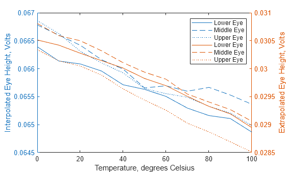
And plot the trends in eye height over temperature.
figure;
yyaxis("left");
plot(tbl.Temperature, tbl.Interpolated);
ylabel("Interpolated Eye Height, Volts");
xlabel("Temperature, degrees Celsius");
yyaxis("right");
plot(tbl.Temperature, tbl.Extrapolated);
ylabel("Extrapolated Eye Height, Volts");
legend("Lower Eye", "Middle Eye", "Upper Eye", "Lower Eye", "Middle Eye", "Upper Eye");