Main Content

lsqr

Solve system of linear equations — least-squares method

Description

example

x = lsqr(A,b) attempts to solve the system of linear equations A*x = b for x using the Least Squares Method. lsqr finds a least squares solution for x that minimizes norm(b-A*x). When A is consistent, the least squares solution is also a solution of the linear system. When the attempt is successful, lsqr displays a message to confirm convergence. If lsqr fails to converge after the maximum number of iterations or halts for any reason, it displays a diagnostic message that includes the relative residual norm(b-A*x)/norm(b) and the iteration number at which the method stopped.

example

x = lsqr(A,b,tol) specifies a tolerance for the method. The default tolerance is 1e-6.

example

x = lsqr(A,b,tol,maxit) specifies the maximum number of iterations to use. lsqr displays a diagnostic message if it fails to converge within maxit iterations.

example

x = lsqr(A,b,tol,maxit,M) specifies a preconditioner matrix M and computes x by effectively solving the system AM1y=b for y, where y=Mx. Using a preconditioner matrix can improve the numerical properties of the problem and the efficiency of the calculation.

example

x = lsqr(A,b,tol,maxit,M1,M2) specifies factors of the preconditioner matrix M such that M = M1*M2.

example

x = lsqr(A,b,tol,maxit,M1,M2,x0) specifies an initial guess for the solution vector x. The default is a vector of zeros.

example

[x,flag] = lsqr(___) returns a flag that specifies whether the algorithm successfully converged. When flag = 0, convergence was successful. You can use this output syntax with any of the previous input argument combinations. When you specify the flag output, lsqr does not display any diagnostic messages.

example

[x,flag,relres] = lsqr(___) also returns the residual error of the computed solution x. If flag is 0, then x is a least-squares solution that minimizes norm(b-A*x). If relres is small, then x is also a consistent solution, since relres represents norm(b-A*x)/norm(b).

example

[x,flag,relres,iter] = lsqr(___) also returns the iteration number iter at which x was computed.

example

[x,flag,relres,iter,resvec] = lsqr(___) also returns a vector of the residual norms at each iteration, including the first residual norm(b-A*x0).

example

[x,flag,relres,iter,resvec,lsvec] = lsqr(___) also returns lsvec, which is an estimate of the scaled normal equation error at each iteration.

Examples

collapse all

Solve a rectangular linear system using lsqr with default settings, and then adjust the tolerance and number of iterations used in the solution process.

Create a random sparse matrix A with 50% density. Also create a random vector b for the right-hand side of Ax=b.

rng default
A = sprand(400,300,.5);
b = rand(400,1);

Solve Ax=b using lsqr. The output display includes the value of the relative residual error b-Axb.

x = lsqr(A,b);
lsqr stopped at iteration 20 without converging to the desired tolerance 1e-06
because the maximum number of iterations was reached.
The iterate returned (number 20) has relative residual 0.26.

By default lsqr uses 20 iterations and a tolerance of 1e-6, but the algorithm is unable to converge in those 20 iterations for this matrix. Since the residual is still large, it is a good indicator that more iterations (or a preconditioner matrix) are needed. You also can use a larger tolerance to make it easier for the algorithm to converge.

Solve the system again using a tolerance of 1e-4 and 70 iterations. Specify six outputs to return the relative residual relres of the calculated solution, as well as the residual history resvec and the least-squares residual history lsvec.

[x,flag,relres,iter,resvec,lsvec] = lsqr(A,b,1e-4,70);
flag
flag = 0

Since flag is 0, the algorithm was able to meet the desired error tolerance in the specified number of iterations. You can generally adjust the tolerance and number of iterations together to make trade-offs between speed and precision in this manner.

Examine the relative residual and least-squares residual of the calculated solution.

relres
relres = 0.2625
lsres = lsvec(end)
lsres = 2.5375e-04

These residual norms indicate that x is a least-squares solution, because relres is not smaller than the specified tolerance of 1e-4. Since no consistent solution to the linear system exists, the best the solver can do is to make the least-squares residual satisfy the tolerance.

Plot the residual histories. The relative residual resvec quickly reaches a minimum and cannot make further progress, while the least-squares residual lsvec continues to be minimized on subsequent iterations.

N = length(resvec);
semilogy(0:N-1,lsvec,'--o',0:N-1,resvec,'-o')
legend("Least-squares residual","Relative residual")

Figure contains an axes object. The axes object contains 2 objects of type line. These objects represent Least-squares residual, Relative residual.

Examine the effect of using a preconditioner matrix with lsqr to solve a linear system.

Load west0479, a real 479-by-479 nonsymmetric sparse matrix.

load west0479
A = west0479;

Define b so that the true solution to Ax=b is a vector of all ones.

b = sum(A,2);

Set the tolerance and maximum number of iterations.

tol = 1e-12;
maxit = 20;

Use lsqr to find a solution at the requested tolerance and number of iterations. Specify six outputs to return information about the solution process:

  • x is the computed solution to A*x = b.

  • fl is a flag indicating whether the algorithm converged.

  • rr is the relative residual of the computed answer x.

  • it is the iteration number when x was computed.

  • rv is a vector of the residual history for b-Ax.

  • lsrv is a vector of the least squares residual history.

[x,fl,rr,it,rv,lsrv] = lsqr(A,b,tol,maxit);
fl
fl = 1
rr
rr = 0.0017
it
it = 20

Since fl = 1, the algorithm did not converge to the specified tolerance within the maximum number of iterations.

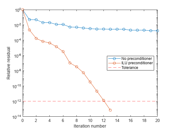
To aid with the slow convergence, you can specify a preconditioner matrix. Since A is nonsymmetric, use ilu to generate the preconditioner M=LU in factorized form. Specify a drop tolerance to ignore nondiagonal entries with values smaller than 1e-6. Solve the preconditioned system AM-1(Mx)=b for y=Mx by specifying L and U as the M1 and M2 inputs to lsqr.

setup = struct('type','ilutp','droptol',1e-6);
[L,U] = ilu(A,setup);
[x1,fl1,rr1,it1,rv1,lsrv1] = lsqr(A,b,tol,maxit,L,U);
fl1
fl1 = 0
rr1
rr1 = 7.1047e-14
it1
it1 = 13

The use of an ilu preconditioner produces a relative residual less than the prescribed tolerance of 1e-12 at the 13th iteration. The output rv1(1) is norm(b), and the output rv1(end) is norm(b-A*x1).

You can follow the progress of lsqr by plotting the relative residuals at each iteration. Plot the residual history of each solution with a line for the specified tolerance.

semilogy(0:length(rv)-1,rv/norm(b),'-o')
hold on
semilogy(0:length(rv1)-1,rv1/norm(b),'-o')
yline(tol,'r--');
legend('No preconditioner','ILU preconditioner','Tolerance','Location','East')
xlabel('Iteration number')
ylabel('Relative residual')

Figure contains an axes object. The axes object with xlabel Iteration number, ylabel Relative residual contains 3 objects of type line, constantline. These objects represent No preconditioner, ILU preconditioner, Tolerance.

Examine the effect of supplying lsqr with an initial guess of the solution.

Create a random rectangular sparse matrix. Use the sum of each row as the vector for the right-hand side of Ax=b so that the expected solution for x is a vector of ones.

A = sprand(700,900,0.1);
b = sum(A,2);

Use lsqr to solve Ax=b twice: one time with the default initial guess, and one time with a good initial guess of the solution. Use 75 iterations and the default tolerance for both solutions. Specify the initial guess in the second solution as a vector with all elements equal to 0.99.

maxit = 75;
x1 = lsqr(A,b,[],maxit);
lsqr converged at iteration 64 to a solution with relative residual 8.7e-07.
x0 = 0.99*ones(size(A,2),1);
x2 = lsqr(A,b,[],maxit,[],[],x0);
lsqr converged at iteration 26 to a solution with relative residual 9.6e-07.

With an initial guess close to the expected solution, lsqr is able to converge in fewer iterations.

Returning Intermediate Results

You also can use the initial guess to get intermediate results by calling lsqr in a for-loop. Each call to the solver performs a few iterations and stores the calculated solution. Then you use that solution as the initial vector for the next batch of iterations.

For example, this code performs 100 iterations four times and stores the solution vector after each pass in the for-loop:

x0 = zeros(size(A,2),1);
tol = 1e-8;
maxit = 100;
for k = 1:4
    [x,flag,relres] = lsqr(A,b,tol,maxit,[],[],x0);
    X(:,k) = x;
    R(k) = relres;
    x0 = x;
end

X(:,k) is the solution vector computed at iteration k of the for-loop, and R(k) is the relative residual of that solution.

Solve a linear system by providing lsqr with a function handle that computes A*x and A'*x in place of the coefficient matrix A.

Create a nonsymmetric tridiagonal matrix. Preview the matrix.

A = gallery('wilk',21) + diag(ones(20,1),1)
A = 21×21

    10     2     0     0     0     0     0     0     0     0     0     0     0     0     0     0     0     0     0     0     0
     1     9     2     0     0     0     0     0     0     0     0     0     0     0     0     0     0     0     0     0     0
     0     1     8     2     0     0     0     0     0     0     0     0     0     0     0     0     0     0     0     0     0
     0     0     1     7     2     0     0     0     0     0     0     0     0     0     0     0     0     0     0     0     0
     0     0     0     1     6     2     0     0     0     0     0     0     0     0     0     0     0     0     0     0     0
     0     0     0     0     1     5     2     0     0     0     0     0     0     0     0     0     0     0     0     0     0
     0     0     0     0     0     1     4     2     0     0     0     0     0     0     0     0     0     0     0     0     0
     0     0     0     0     0     0     1     3     2     0     0     0     0     0     0     0     0     0     0     0     0
     0     0     0     0     0     0     0     1     2     2     0     0     0     0     0     0     0     0     0     0     0
     0     0     0     0     0     0     0     0     1     1     2     0     0     0     0     0     0     0     0     0     0
      ⋮

Since this tridiagonal matrix has a special structure, you can represent the operation A*x with a function handle. When A multiplies a vector, most of the elements in the resulting vector are zeros. The nonzero elements in the result correspond with the nonzero tridiagonal elements of A.

The expression Ax becomes:

Ax=[1020019200120010010200110][x1x2x3x21]=[10x1+2x2x1+9x2+2x3x19+9x20+2x21x20+10x21].

The resulting vector can be written as the sum of three vectors:

Ax=[10x1+2x2x1+9x2+2x3x19+9x20+2x21x20+10x21]=[0x1x2x20]+[10x19x29x2010x21]+2[x2x3x210].

Likewise, the expression for ATx becomes:

ATx=[1010029100210020010100210][x1x2x3x21]=[10x1+x22x1+9x2+x32x19+9x20+x212x20+10x21].

ATx=[10x1+x22x1+9x2+x32x19+9x20+x212x20+10x21]=2[0x1x2x20]+[10x19x29x2010x21]+[x2x3x210].

In MATLAB®, write a function that creates these vectors and adds them together, thus giving the value of A*x or A'*x, depending on the flag input:

function y = afun(x,flag)
if strcmp(flag,'notransp') % Compute A*x
    y = [0; x(1:20)] ...
        + [(10:-1:0)'; (1:10)'].*x ...
        + 2*[x(2:end); 0];
elseif strcmp(flag,'transp') % Compute A'*x
    y = 2*[0; x(1:20)] ...
        + [(10:-1:0)'; (1:10)'].*x ...
        + [x(2:end); 0];
end
end

(This function is saved as a local function at the end of the example.)

Now, solve the linear system Ax=b by providing lsqr with the function handle that calculates A*x and A'*x. Use a tolerance of 1e-6 and 25 iterations. Specify b as the row sums of A so that the true solution for x is a vector of ones.

b = full(sum(A,2));
tol = 1e-6;  
maxit = 25;
x1 = lsqr(@afun,b,tol,maxit)
lsqr converged at iteration 21 to a solution with relative residual 4.5e-12.
x1 = 21×1

    1.0000
    1.0000
    1.0000
    1.0000
    1.0000
    1.0000
    1.0000
    1.0000
    1.0000
    1.0000
      ⋮

Local Functions

function y = afun(x,flag)
if strcmp(flag,'notransp') % Compute A*x
    y = [0; x(1:20)] ...
        + [(10:-1:0)'; (1:10)'].*x ...
        + 2*[x(2:end); 0];
elseif strcmp(flag,'transp') % Compute A'*x
    y = 2*[0; x(1:20)] ...
        + [(10:-1:0)'; (1:10)'].*x ...
        + [x(2:end); 0];
end
end

Input Arguments

collapse all

Coefficient matrix, specified as a matrix or function handle. This matrix is the coefficient matrix in the linear system A*x = b. Generally, A is a large sparse matrix or a function handle that returns the product of a large sparse matrix and column vector.

Specifying A as a Function Handle

You can optionally specify the coefficient matrix as a function handle instead of a matrix. The function handle returns matrix-vector products instead of forming the entire coefficient matrix, making the calculation more efficient.

To use a function handle, use the function signature function y = afun(x,opt). Parameterizing Functions explains how to provide additional parameters to the function afun, if necessary. The function afun must satisfy these conditions:

  • afun(x,'notransp') returns the product A*x.

  • afun(x,'transp') returns the product A'*x.

An example of an acceptable function is:

function y = afun(x,opt,B,C,n)
if strcmp(opt,'notransp')
    y = [B*x(n+1:end); C*x(1:n)];
else
    y = [C'*x(n+1:end); B'*x(1:n)];
end
The function afun uses the values in B and C to compute either A*x or A'*x (depending on the specified flag) without actually forming the entire matrix.

Data Types: double | function_handle
Complex Number Support: Yes

Right-hand side of linear equation, specified as a column vector. The length of b must be equal to size(A,1).

Data Types: double
Complex Number Support: Yes

Method tolerance, specified as a positive scalar. Use this input to trade-off accuracy and runtime in the calculation. lsqr must meet the tolerance within the number of allowed iterations to be successful. A smaller value of tol means the answer must be more precise for the calculation to be successful.

Data Types: double

Maximum number of iterations, specified as a positive scalar integer. Increase the value of maxit to allow more iterations for lsqr to meet the tolerance tol. Generally, a smaller value of tol means more iterations are required to successfully complete the calculation.

Preconditioner matrices, specified as separate arguments of matrices or function handles. You can specify a preconditioner matrix M or its matrix factors M = M1*M2 to improve the numerical aspects of the linear system and make it easier for lsqr to converge quickly. For square coefficient matrices, you can use the incomplete matrix factorization functions ilu and ichol to generate preconditioner matrices. You also can use equilibrate prior to factorization to improve the condition number of the coefficient matrix. For more information on preconditioners, see Iterative Methods for Linear Systems.

lsqr treats unspecified preconditioners as identity matrices.

Specifying M as a Function Handle

You can optionally specify any of M, M1, or M2 as function handles instead of matrices. The function handle performs matrix-vector operations instead of forming the entire preconditioner matrix, making the calculation more efficient.

To use a function handle, first create a function with the signature function y = mfun(x,opt). Parameterizing Functions explains how to provide additional parameters to the function mfun, if necessary. The function mfun must satisfy these conditions:

  • mfun(x,'notransp') returns the value of M\x or M2\(M1\x).

  • mfun(x,'transp') returns the value of M'\x or M1'\(M2'\x).

An example of an acceptable function is:

function y = mfun(x,opt,a,b)  
if strcmp(opt,'notransp')
    y = x.*a;
else
    y = x.*b;
end
end
In this example the function mfun uses a and b to compute either M\x = x*a or M'\x = x*b (depending on the specified flag) without actually forming the entire matrix M.

Data Types: double | function_handle
Complex Number Support: Yes

Initial guess, specified as a column vector with length equal to size(A,2). If you can provide lsqr with a more reasonable initial guess x0 than the default vector of zeros, then it can save computation time and help the algorithm converge faster.

Data Types: double
Complex Number Support: Yes

Output Arguments

collapse all

Linear system solution, returned as a column vector. This output gives the approximate solution to the linear system A*x = b.

  • If flag is 0 and relres <= tol, then x is a consistent solution to A*x = b.

  • If flag is 0 but relres > tol, then x is the least squares solution that minimizes norm(b-A*x). In this case, the lsvec output contains the scaled normal equation error of x.

Whenever the calculation is not successful (flag ~= 0), the solution x returned by lsqr is the one with minimal norm residual computed over all the iterations.

Convergence flag, returned as one of the scalar values in this table. The convergence flag indicates whether the calculation was successful and differentiates between several different forms of failure.

Flag Value

Convergence

0

Success — lsqr converged to the desired tolerance tol within maxit iterations.

1

Failure — lsqr iterated maxit iterations but did not converge.

2

Failure — The preconditioner matrix M or M = M1*M2 is ill conditioned.

3

Failure — lsqr stagnated after two consecutive iterations were the same.

4

Failure — One of the scalar quantities calculated by the lsqr algorithm became too small or too large to continue computing.

Relative residual error, returned as a scalar. The relative residual error is an indication of how accurate the returned answer x is. lsqr tracks the relative residual and least-squares residual at each iteration in the solution process, and the algorithm converges when either residual meets the specified tolerance tol. The relres output contains the value of the residual that converged, either the relative residual or the least-squares residual:

  • The relative residual error is equal to norm(b-A*x)/norm(b) and is generally the residual that meets the tolerance tol when lsqr converges. The resvec output tracks the history of this residual over all iterations.

  • The least-squares residual error is equal to norm((A*inv(M))'*(B-A*X))/norm(A*inv(M),'fro'). This residual causes lsqr to converge less frequently than the relative residual. The lsvec output tracks the history of this residual over all iterations.

Iteration number, returned as a scalar. This output indicates the iteration number at which the computed answer for x was calculated.

Data Types: double

Residual error, returned as a vector. The residual error norm(b-A*x) reveals how close the algorithm is to converging for a given value of x. The number of elements in resvec is equal to the number of iterations. You can examine the contents of resvec to help decide whether to change the values of tol or maxit.

Data Types: double

Scaled normal equation error, returned as a vector. For each iteration, lsvec contains an estimate of the scaled normal equation residual norm((A*inv(M))'*(B-A*X))/norm(A*inv(M),'fro'). The number of elements in lsvec is equal to the number of iterations.

More About

collapse all

Least Squares Method

The least squares (LSQR) algorithm is an adaptation of the conjugate gradients (CG) method for rectangular matrices. Analytically, LSQR for A*x = b produces the same residuals as CG for the normal equations A'*A*x = A'*b, but LSQR possesses more favorable numeric properties and is thus generally more reliable [1].

The least squares method is the only iterative linear system solver that can handle rectangular and inconsistent coefficient matrices.

Tips

  • Convergence of most iterative methods depends on the condition number of the coefficient matrix, cond(A). When A is square, you can use equilibrate to improve its condition number, and on its own this makes it easier for most iterative solvers to converge. However, using equilibrate also leads to better quality preconditioner matrices when you subsequently factor the equilibrated matrix B = R*P*A*C.

  • You can use matrix reordering functions such as dissect and symrcm to permute the rows and columns of the coefficient matrix and minimize the number of nonzeros when the coefficient matrix is factored to generate a preconditioner. This can reduce the memory and time required to subsequently solve the preconditioned linear system.

References

[1] Barrett, R., M. Berry, T. F. Chan, et al., Templates for the Solution of Linear Systems: Building Blocks for Iterative Methods, SIAM, Philadelphia, 1994.

[2] Paige, C. C. and M. A. Saunders, "LSQR: An Algorithm for Sparse Linear Equations And Sparse Least Squares," ACM Trans. Math. Soft., Vol.8, 1982, pp. 43-71.

Extended Capabilities

Version History

Introduced before R2006a