Ground State of Hydrogen Molecule Using Variational Quantum Eigensolver (VQE)

This example shows how to implement a variational quantum eigensolver (VQE) to estimate the ground state of the hydrogen molecule ${\mathit{H}}_2$. VQE is a hybrid algorithm that uses both quantum circuits and classical optimization to solve eigenvalue problems, such as finding the lowest energy state of a molecule. The VQE algorithm, based on the Rayleigh–Ritz variational principle, uses a parameterized quantum circuit to represent the trial wavefunction (ansatz) of a molecule and quantum measurements to obtain the expectation value of the molecular Hamiltonian. A classical optimizer iteratively updates the circuit parameters to minimize this expectation value, thereby approximating the ground-state energy of the molecular system.

Formulate Cost Function to Minimize

In a molecular system, you typically apply the Jordan–Wigner transformation to decompose the Hamiltonian operator into a linear combination of multiqubit Pauli operators [1]:

$\mathit{H}\left(\mathit{R}\right)={\sum }_{\mathit{j}}{\mathit{h}}_{\mathit{j}}\left(\mathit{R}\right){\prod }_{\mathit{i}}^{\mathit{N}}{\sigma }_{\mathit{i}}^{\mathit{j}}$.

In this Hamiltonian, the parameters $\mathit{R}$ are related to the geometry (the nuclear coordinates of the molecule), and ${\mathit{h}}_{\mathit{j}}\left(\mathit{R}\right)$ are expansion coefficients that depend on those parameters. The operators ${\sigma }_{\mathit{i}}$ are elements of the Pauli group $\left\{\mathit{I},\mathit{X},\mathit{Y},\mathit{Z}\right\}$, and $\mathit{N}$ is the number of qubits.

To find the ground state of the molecule, define the cost function to minimize as the expectation value of the parameterized Hamiltonian $\mathit{H}\left(\mathit{R}\right)$:

$\mathit{E}\left(\Theta ,\mathit{R}\right)=\left.anglebracketleft\Psi \left(\Theta \right)\right|\mathit{H}\left(\mathit{R}\right)\left|\Psi \left(\Theta \right)\right.anglebracketright$.

Here, $\left|\Psi \left(\Theta \right)\right.anglebracketright$ is the $\mathit{N}$-qubit trial wavefunction of the molecule, which can be represented by a quantum circuit for a given set of parameters $\Theta$. The VQE algorithm solves the optimization problem

$\underset{\left\{\Theta ,\mathit{R}\right\}}{\min }\mathit{E}\left(\Theta ,\mathit{R}\right)$.

This cost function depends on both the circuit parameters $\Theta$ and the Hamiltonian parameters $\mathit{R}$, which are minimized using a classical optimization scheme. At each iteration, the optimization computes updated values for $\Theta$ and $\mathit{R}$, which the quantum circuit then uses to measure the updated cost function. Iterations continue until a defined stopping point or specific criteria for convergence are met.

Create Hamiltonian for Hydrogen Molecule

To find the ground state of the ${\mathit{H}}_2$ molecule, this example users a predetermined Hamiltonian chosen for a bond distance of 0.742 Å. In other words, the parameters $\mathit{R}$ corresponding to the bond distance are fixed to simplify the optimization problem. The quantum circuit that describes the Hamiltonian uses four qubits, based on table II of [2].

PauliTerms = ["IIII"; "ZIII"; "IZII"; ...
              "ZZII"; "IIZI"; "ZIZI"; ...
              "IIIZ"; "ZIIZ"; "IZZI"; ...
              "IZIZ"; "IIZZ"; "YXXY"; ...
              "XYYX"; "XXYY"; "YYXX"];
Coefficients = [-0.09963387941370971; ...
                 0.17110545123720233; ...
                 0.17110545123720233; ...
                 0.16859349595532533; ...
                -0.22250914236600539; ...
                 0.12051027989546245; ...
                -0.22250914236600539; ...
                 0.16584090244119712; ...
                 0.16584090244119712; ...
                 0.12051027989546245; ...
                 0.17432077259242010; ...
                 0.04533062254573469; ...
                 0.04533062254573469; ...
                -0.04533062254573469; ...
                -0.04533062254573469];

Represent the Hamiltonian in the multiqubit Pauli basis by using the observable function.

Hamiltonian = observable(PauliTerms,Coefficients)

Hamiltonian = 
  observable with properties:

       Paulis: [15×1 string]
      Weights: [15×1 double]
    NumQubits: 4

Create Parameterized Circuit for Trial Wavefunction

In this example, a double excitation gate parameterizes the trial wavefunction. The double excitation gate is created based on figure 11 of [5], where the gate performs this transformation:

$$\begin{array}{l}\left|0011\right.anglebracketright\to \cos \left(\frac{\theta }{2}\right)\left|0011\right.anglebracketright+\sin \left(\frac{\theta }{2}\right)\left|1100\right.anglebracketright\\ \left|1100\right.anglebracketright\to \cos \left(\frac{\theta }{2}\right)\left|1100\right.anglebracketright-\sin \left(\frac{\theta }{2}\right)\left|0011\right.anglebracketright\end{array}$$

For the ${\mathit{H}}_2$ molecule, formulate the wavefunction to optimize as

$\Psi \left(\theta \right)=\cos \left(\frac{\theta }{2}\right)\left|1100\right.anglebracketright-\sin \left(\frac{\theta }{2}\right)\left|0011\right.anglebracketright$.

Here, the wavefunction depends on a single parameter $\theta$. The first term of the wavefunction $\left|1100\right.anglebracketright$, which represents the Hartree–Fock state, describes the two electrons in the molecule occupying the lowest-energy orbitals. The second term $\left|0011\right.anglebracketright$ represents a double excitation, in which the electrons are excited from qubits 1 and 2 to qubits 3 and 4. The VQE algorithm optimizes the parameter $\theta$ to find the ground state of the molecule.

Create the gates and quantum circuit that represent the wavefunction in a helper function. The doubleExcitationGate helper function takes the angle parameter $\theta$ as an input.

function circuit = doubleExcitationGate(theta)
  initGates = xGate([1 2]);
  gatesComposition = [cxGate(3,4); cxGate(1,3); hGate([1 4]); ...
    cxGate(1,2); cxGate(3,4); ryGate(1,-theta/8); ...
    ryGate(2,theta/8); cxGate(1,4); hGate(4); cxGate(4,2); ...
    ryGate(1,-theta/8); ryGate(2,theta/8); cxGate(3,2); ...
    cxGate(3,1); ryGate(1,theta/8); ryGate(2,-theta/8); ...
    cxGate(4,2); hGate(4); cxGate(1,4); ryGate(1,theta/8); ...
    ryGate(2,-theta/8); cxGate(1,2); cxGate(3,1); ...
    hGate([1 4]); cxGate(1,3); cxGate(3,4)];
  circuit = quantumCircuit([initGates; gatesComposition]);
end

Define Function to Measure Energy

Next, define the expectation function that measures the energy of the ${\mathit{H}}_2$ molecule. This function takes the Hamiltonian, the $\theta$ parameter, and the logical QPUrun option as inputs. By default, the QPUrun option is set to false, where the energy measurement is performed using a local simulation. If QPUrun is set to true, the energy measurement is performed using a remote quantum processing unit (QPU) provided by the IBM® device "ibm_fez".

To run quantum circuits on an IBM quantum device from within MATLAB, you need an IBM account with access to the Qiskit® Runtime service. For more information, see Run Quantum Circuit on Hardware Using IBM Qiskit Runtime Service.

To measure the energy or expectation value of the quantum circuit in the Pauli basis specified by the Hamiltonian using a QPU, use the run function and specify the Observable argument as the Hamiltonian. To measure the energy using a local simulation instead, use the observe function. The expectation function returns the measured energy as the first output argument. If you specify a second output argument, then the expectation function also returns the trial wavefunction for the specified $\theta$ parameter.

function varargout = expectation(Hamiltonian,theta,opts)
  arguments
    Hamiltonian
    theta
    opts.QPUrun (1,1) logical = false
  end  

  devIBM = quantum.backend.QuantumDeviceIBM("ibm_fez");
  circuit = doubleExcitationGate(theta);

  if opts.QPUrun
    task = run(circuit,devIBM,Observable=Hamiltonian);
    wait(task);
    energy = fetchOutput(task);
  else
    energy = observe(circuit,Hamiltonian);
  end

  if nargout == 1
      varargout{1} = energy;
  elseif nargout == 2
      varargout{1} = energy;
      varargout{2} = formula(simulate(circuit));
  end
end

Find Minimum Energy Using Exhaustive Search Method

To find the minimum energy, you can first use the exhaustive search method by specifying a range of values for $\theta$ and computing the energy at each value. Although this method is slow, it is easy to understand and serves well for benchmarking purposes. Plot the energy as a function of the angle parameter $\theta$.

theta = -0.5:0.001:1;
e = zeros(size(theta));
w = createArray(size(theta),"string");
for i = 1:length(theta)
  [e(i),w(i)] = expectation(Hamiltonian,theta(i));
end

The availability of IBM quantum computing systems for submission of quantum inputs 
by you (the End User) is provided AS IS and is limited to experimental research, 
education, testing, evaluation and feedback purposes by End Users, and no commercial or 
production use by End Users is permitted. Results are not guaranteed.

figure;
plot(theta,e)
xlabel("Angle Parameter $\theta$ (rad)",Interpreter="latex")
ylabel("$H_2$ Energy (hartrees)",Interpreter="latex")

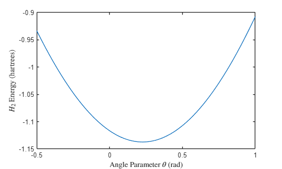
Find the minimum energy and the corresponding value of $\theta$. Show the value of $\theta$ and the wavefunction that minimize the energy. Using this method, the minimum energy is –1.1373 hartrees and the $\theta$ angle is 0.226 rad.

[minEnergy,id] = min(e)

minEnergy = 
-1.1373

id = 
727

minTheta = theta(id)

minTheta = 
0.2260

minWavefunction = w(id)

minWavefunction = 
    "-0.11276 * |0011> +
     0.99362  * |1100>"

Find Minimum Energy Using Gradient-Descent Method

To find the minimum energy, you can use the gradient-descent optimization method. In this section, you optimize the expectation function using the gradient-descent method, locally simulating the parametrized circuit and then running it on a QPU.

Define Gradient-Descent Method

To implement the gradient-descent method, first formulate the gradient for the cost function, or the energy. Here, the gradient has an analytical formula based on the parameter-shift rule, which is equation 30 of [5]:

$\frac{\partial \mathit{E}\left(\theta \right)}{\partial \theta }=\frac{\mathit{E}\left(\theta +\mathit{s}\right)-\mathit{E}\left(\theta -\mathit{s}\right)}{2\sin \left(\mathit{s}\right)}$.

Define the expectationGradient function that computes this gradient using the specified value of $\mathit{s}=\pi /2$.

function grad = expectationGradient(Hamiltonian,theta,opts)
  arguments
    Hamiltonian
    theta
    opts.QPUrun (1,1) logical = false
  end
  
  s = pi/2;
  grad = (expectation(Hamiltonian,theta+s,QPUrun=opts.QPUrun) - ...
          expectation(Hamiltonian,theta-s,QPUrun=opts.QPUrun))/2/sin(s);
end

Next, define the gradientDescent function that performs the gradient-descent optimization. This function measures the energy and its gradient in each iteration. During the iteration process, these measurements are used to update the lowest measured energy, and the sgdmupdate function updates the learnable parameters in the gradient-descent method. The iterations stop when the learnable velocity parameter converges within the specified tolerance or when the maximum number of iterations is reached.

function [theta_optimal,cost_history] = gradientDescent(theta_init,cost_function,gradient,options)
  % Extract options  
  lr = options.learning_rate;
  max_iter = options.max_iterations;
  mu = options.momentum;
  tol = options.tolerance;
  
  % Initialize variables
  theta_current = theta_init;
  velocity = [];
  cost_history = [];
  best_cost = Inf;
  best_theta = theta_current;
    
  for iter = 1:max_iter
    % Compute current cost function and gradient
    current_cost = cost_function(theta_current);
    current_grad = gradient(theta_current);
    cost_history(iter) = current_cost;
    
    % Update best solution if current cost is lower
    if current_cost < best_cost
      best_cost = current_cost;
      best_theta = theta_current;
    end
    
    % Update learnable parameters using sgdmupdate
    [theta_current,velocity] = sgdmupdate(theta_current,current_grad,velocity,lr,mu);
    
    % Check convergence
    if norm(velocity) < tol
      break;
    end
  end
    
  theta_optimal = best_theta;
  disp("Optimization stops at iteration no." + string(iter))
end

Compute Ground State Energy Using Local Simulation

Define the options for the gradient-descent optimization. Specify the initial guess of the search parameter as $\theta =1$. Set the learning rate to 0.02, the maximum number of iterations to 200, the momentum to 0.8, and the tolerance to 1e-6.

theta_init = 1;
options = struct("learning_rate",0.02, ...
                 "max_iterations",200, ...
                 "momentum",0.8, ...
                 "tolerance",1e-6);

Perform the gradient-descent optimization using local simulation.

[theta_optimal,cost_history] = gradientDescent(theta_init, ...
    @(theta) expectation(Hamiltonian,theta), ...
    @(theta) expectationGradient(Hamiltonian,theta), ...
    options);

Optimization stops at iteration no.85

Plot the optimization progress.

figure;
plot(cost_history,"bo");
xlabel("Iteration");
ylabel("Cost Function");
title("Optimization Progress (Local Simulation)");

Show the minimum energy and the corresponding value of $\theta$.

minEnergy = cost_history(end)

minEnergy = 
-1.1373

minTheta = theta_optimal

minTheta = 
0.2264

The optimizer stops when the learnable velocity parameter converges within the specified tolerance, after 85 iterations. Here, the cost function and the angle parameter also converge within some bounds. The result obtained using the gradient-descent method with local simulation is consistent with the result from the exhaustive search method. The ground state energy of the ${\mathit{H}}_2$ molecule is –1.1373 hartrees, and the corresponding $\theta$ angle is 0.2264 rad.

Compute Ground State Energy Using QPU

To perform the gradient-descent optimization using a QPU, use the gradientDescent function with the QPUrun argument set to true. For example, you can perform the optimization on a QPU using previous options defined for local simulation.

[theta_optimal,cost_history] = gradientDescent(theta_init, ...
    @(theta) expectation(Hamiltonian,theta,QPUrun=true), ...
    @(theta) expectationGradient(Hamiltonian,theta,QPUrun=true), ...
    options);

Running this optimization on a QPU can take some time due to the queue time required to run a new task each time the angle parameter is updated.

You can also measure the ground state energy of the ${\mathit{H}}_2$ molecule on a QPU using the angle parameter obtained from the local simulation.

energy = expectation(Hamiltonian,minTheta,QPUrun=true)

energy = 
-0.8445

Because of the noise in physical quantum devices, the ground state energy measured using the QPU differs from that obtained in local simulations.

References

[1] Delgado, Alain, Juan M. Arrazola, Soran Jahangiri, Zeyue Niu, Josh Izaac, Chase Roberts, and Nathan Killoran. "Variational Quantum Algorithm for Molecular Geometry Optimization." Physical Review A 104, no. 5 (November 2, 2021): 052402. https://doi.org/10.1103/PhysRevA.104.052402.

[2] Pankkonen, Joona V., Lauri Ylinen, Matti Raasakka, and Ilkka Tittonen. "Improving Variational Quantum Circuit Optimization via Hybrid Algorithms and Random Axis Initialization." arXiv, March 26, 2025. https://doi.org/10.48550/arXiv.2503.20728.

[3] Symeonidou, Stefania-Rebekka. "The Variational Quantum Eigensolver in Quantum Chemistry with PennyLane." Bachelor's thesis, RWTH Aachen University, Germany, 2023. https://fz-juelich.sciebo.de/s/2gMTwZZ9FCixi7C.

[4] Anselmetti, Gian-Luca R., David Wierichs, Christian Gogolin, and Robert M. Parrish. "Local, Expressive, Quantum-Number-Preserving VQE Ansätze for Fermionic Systems." New Journal of Physics 23, no.11 (November 12, 2021): 113010. https://doi.org/10.1088/1367-2630/ac2cb3.

[5] Arrazola, Juan M., Olivia Di Matteo, Nicolás Quesada, Soran Jahangiri, Alain Delgado, and Nathan Killoran. "Universal Quantum Circuits for Quantum Chemistry." Quantum 6 (June 20, 2022): 742. https://doi.org/10.22331/q-2022-06-20-742.