Hurricane Natural Catastrophe Risk Estimation

Since R2025a

This example measures natural catastrophe (NatCat) risk for hurricanes in an area of interest (AOI) by using simulations from a hazard model, data about property assets, and a damage function.

Hurricanes are a common natural catastrophe and a key focus for NatCat modeling in the insurance industry. Traditionally, NatCat models measure financial risk by combining three inputs [7]:

• Data related to a hazard of interest. For this example, the hazard data comes from hurricane simulations [2] generated from the approach used in [1].

• Data related to a set of exposures. For this example, the exposure data includes the addresses of several property assets, the geographic locations of the property assets, and the median values of surrounding property assets.

• Information related to asset vulnerability. Asset vulnerability is typically calculated using a damage function, which estimates damage by combining an intensity metric with data about the asset. For this example, the intensity metric is wind speed.

NatCat risk models typically cover a short time period, often a year. A related risk model, physical climate risk, measures NatCat risk using multiple long-term climate scenarios, then models the impact of the long-term risk on financial variables such as house prices and insurance costs. Physical risk models typically cover longer time periods, often decades. As a result, NatCat risk models are useful in isolation and for physical risk models.

Within the example, you perform these tasks:

• Import, process, and visualize the hurricane simulations.

• Specify the exposure data using the addresses of properties in Florida.

• Define a damage function.

• Estimate property loss using the hurricane simulations, the exposure data, and the damage function.

• Analyze the property loss for individual properties and for a portfolio of properties.

Import and Process Hurricane Data

Import and process a file that contains simulated hurricane data [2] generated from the approach used in [1]. The data represents 1000 possible scenarios in the North Atlantic basin for the year 2021, where each simulated year contains zero to multiple hurricanes.

Create a temporary folder to store a text file containing hurricane data. Download the file into the folder by using the downloadHurricaneData helper function. The helper function is attached to the example as a supporting file.

dataDir = fullfile(tempdir,"HurricaneData");
if ~exist(dataDir,"dir")
    mkdir(dataDir)
end
downloadHurricaneData(dataDir)

Specify the name of the text file. Then, read the data into the workspace as a table. View the top rows of the table.

filename = fullfile(dataDir,"HurricaneData.txt");
hcanes = readtable(filename);
head(hcanes)

    Landfall    Latitude    Longitude    MaximumWindSpeed    MinimumPressure    RadiusToMaximumWinds    TCnumber    TimeStep    Year
    ________    ________    _________    ________________    _______________    ____________________    ________    ________    ____

       0          8.9         314.8           20.372             993.95                  46.3              0           0         0  
       0            9         314.3             21.2              992.8                45.906              0           1         0  
       0          9.1         313.6             21.7              992.1                45.512              0           2         0  
       0          9.2         312.7             21.1                993                45.118              0           3         0  
       0          9.3         311.7             20.9              993.1                44.724              0           4         0  
       0          9.5         310.7             21.2              992.7                 44.33              0           5         0  
       0          9.7         309.6             20.8              993.3                43.936              0           6         0  
       0          9.9         308.5             20.3              993.9                43.542              0           7         0  

Each table row represents a hurricane center during a three-hour interval. The table includes these variables:

• Landfall — Indicates if the hurricane center makes landfall.

• Latitude and Longitude — Latitude-longitude coordinates of the hurricane center.

• MaximumWindSpeed — Maximum wind speed, in m/s.

• MinimumPressure — Minimum pressure, in hPa.

• RadiusToMaximumWinds —Radius to maximum winds, in km.

• TCnumber — Hurricane ID for the simulation year.

• TimeStep — Time interval number.

• Year — Simulation year. Each value of Year represents a simulation for 2021. When combined, the Year and TCnumber variables identify unique hurricanes.

Many Mapping Toolbox™ functions require you to use geospatial tables as input. A geospatial table is a table with a Shape variable that contains point, line, or polygon shapes. To convert the table to a geospatial table:

• Create point shapes from the latitude-longitude coordinates. Wrap the longitudes to the range [–180, 180].

• Add a Shape table variable that stores the point shapes.

• Remove the Latitude and Longitude table variables.

Shape = geopointshape(hcanes.Latitude,wrapTo180(hcanes.Longitude));
hcanes = addvars(hcanes,Shape,Before=1);
hcanes = removevars(hcanes,["Latitude","Longitude"]);

Prepare to visualize the hurricane data by creating a subtable of hurricane centers for an area of interest (AOI) surrounding Florida. To simplify the visualization, include only the hurricane centers that make landfall.

• Get an AOI for Florida by using the geocode function. The geocode function represents the AOI using a polygon shape in geographic coordinates.

• Ensure that the AOI contains relevant analysis data by adding a buffer of 100 km.

• Find the table rows for the hurricanes that make landfall in Florida. Create a subtable from the rows.

florida = geocode("Florida");
aoi = florida.Shape;

aoi = buffer(aoi,km2deg(100));

isfloridalandhcane = isinterior(aoi,Shape) & hcanes.Landfall;
floridalandhcanes = hcanes(isfloridalandhcane,:);

Analyze the variation in hurricane size within the AOI by displaying the minimum, maximum, and average values for RadiusToMaximumWinds.

[MinRadius,MaxRadius] = bounds(floridalandhcanes.RadiusToMaximumWinds);
MeanRadius = mean(floridalandhcanes.RadiusToMaximumWinds);
hcanestats = table(MinRadius,MaxRadius,MeanRadius);
disp(hcanestats)

    MinRadius    MaxRadius    MeanRadius
    _________    _________    __________

      9.26        203.72        52.582  

Visualize Hurricane Data

Visualize the data by displaying the hurricane tracks on maps. Create an initial map using all the hurricane data. Then, create a more focused map by displaying the data for one sample hurricane.

Visualize All Hurricane Tracks

Create a map that uses a topographic basemap.

figure
geobasemap topographic
hold on

For a given hurricane track, the table rows have matching Year and TCnumber values. As a result, you can display a line for each track by iterating through the unique values of Year and TCnumber. Create the lines by using the geoplot function and the latitude-longitude coordinates of the hurricane centers. Mark each hurricane center with an asterisk.

% Iterate through unique Year values
years = unique(floridalandhcanes.Year);
for year = years'
    yearhcanes = floridalandhcanes(floridalandhcanes.Year == year,:);
    % Iterate through unique TCnumber values
    TCnums = unique(yearhcanes.TCnumber);
    for TCnum = TCnums'
        hcane = yearhcanes(yearhcanes.TCnumber == TCnum,:);
        % Plot hurricane track using a line
        geoplot(hcane.Shape.Latitude,hcane.Shape.Longitude,"-*")
    end
end

Set the latitude and longitude limits of the map using the bounds of the AOI. Add a title.

[latlim,lonlim] = bounds(aoi);
geolimits(latlim,lonlim)
title("All Hurricane Tracks")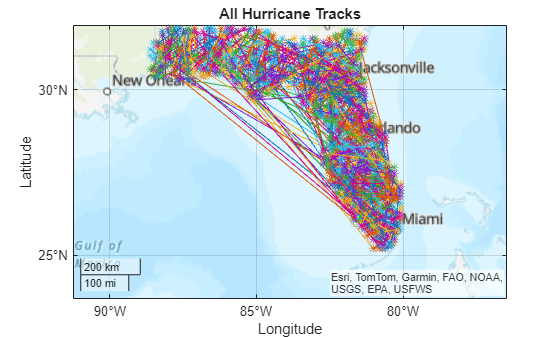

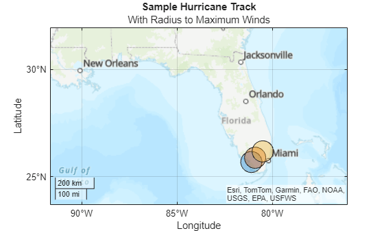
Visualize Sample Hurricane

Create a subtable that contains the hurricane centers for one sample hurricane, in this case the 10th hurricane to occur during the 32nd simulation year.

sampleYear = 32;
sampleTCnum = 10;
sampleind = floridalandhcanes.TCnumber==sampleTCnum & floridalandhcanes.Year==sampleYear;
samplehcane = floridalandhcanes(sampleind,:);

Display the subtable. Note that the radius to maximum winds is approximately 55.56 km, which is close to the average radius of 52.582 km.

samplehcane

samplehcane=3×8 table
            Shape             Landfall    MaximumWindSpeed    MinimumPressure    RadiusToMaximumWinds    TCnumber    TimeStep    Year
    ______________________    ________    ________________    _______________    ____________________    ________    ________    ____

    (25.7000°N, 81.1000°W)       1              19.9                 995                55.56               10           8        32 
    (25.9000°N, 80.9000°W)       1              19.3                 996                55.56               10           9        32 
    (26.2000°N, 80.5000°W)       1              18.6               997.1                55.56               10          10        32 

Create a new map. Then, for each time interval, create and display a circular AOI that represents the radius to maximum winds. The map shows that the sample hurricane makes landfall during three time steps.

figure
geobasemap topographic
hold on

for rowind = 1:height(samplehcane)
    hcanestep = samplehcane(rowind,:);
    stepcircle = aoicircle(hcanestep.Shape,km2deg(hcanestep.RadiusToMaximumWinds));
    geoplot(stepcircle)
end

geolimits(latlim,lonlim)
title("Sample Hurricane Track")
subtitle("With Radius to Maximum Winds")

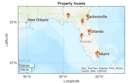
Specify and Visualize Property Assets

Specify the exposure data using the addresses of several property assets, the geographic locations of the property assets, and the median values of surrounding property assets.

Create a list of addresses for several properties in Florida. The list includes three properties in each of these cities: Tallahassee, Tampa, Jacksonville, Gainesville, Miami, and Orlando.

addresses = ["911 Easterwood Dr, Tallahassee, FL" ...
    "3226 Flastacowo Rd, Tallahassee, FL" ...
    "3840 N Monroe St, Tallahassee, FL" ...
    "5300 Interbay Blvd, Tampa, FL" ...
    "3804 E 26th Ave, Tampa, FL" ...
    "11001 N 15th St, Tampa, FL" ...
    "370 Zoo Pkwy, Jacksonville, FL" ...
    "117 W Duval St, Jacksonville, FL" ...
    "3625 University Blvd S, Jacksonville, FL" ...
    "224 SE 24th St, Gainesville, FL" ...
    "803 NW 192nd Ave, Gainesville, FL" ...
    "309 Village Dr, Gainesville, FL" ...
    "11805 SW 26th St, Miami, FL" ...
    "3500 Pan American Dr, Miami, FL" ...
    "11380 NW 27th Ave, Miami, FL" ...
    "5100 L B McLeod Rd, Orlando, FL" ...
    "595 N Primrose Dr, Orlando, FL" ...
    "6501 Magic Way, Orlando, FL"];

Create a table that stores information about the property assets. Then, create a table row for each address by using the geocode function. The function represents the locations of the addresses using point shapes in geographic coordinates.

assets = table;
for address = addresses
    newRow = geocode(address,"address",FilterResults="first");
    assets = [assets; newRow]; %#ok<AGROW>
end

Prepare to calculate property damages and losses by adding two variables to the table:

• AssetValues estimates the median house price for each city.

• DistanceToSea estimates the distance, in km, from each city to the sea.

Note that, while median house prices and approximate distances are appropriate for illustrative purposes, you can create more accurate risk models by using more specific data.

AssetValues = zeros(numel(addresses),1);
AssetValues(1:3) = 554500;   % Tallahassee
AssetValues(4:6) = 460000;   % Tampa
AssetValues(7:9) = 301000;   % Jacksonville
AssetValues(10:12) = 315000; % Gainesville
AssetValues(13:15) = 699000; % Miami
AssetValues(16:18) = 399000; % Orlando

DistanceToSea = zeros(numel(addresses),1);
DistanceToSea(1:3) = 35;   % Tallahassee
DistanceToSea(4:6) = 5;    % Tampa
DistanceToSea(7:9) = 20;   % Jacksonville
DistanceToSea(10:12) = 80; % Gainesville
DistanceToSea(13:15) = 5;  % Miami
DistanceToSea(16:18) = 55; % Orlando

assets = addvars(assets,AssetValues,DistanceToSea);

View the first two rows of the assets table.

head(assets,2)

            Shape                                   Name                           AdminLevel    AssetValues    DistanceToSea
    ______________________    _________________________________________________    __________    ___________    _____________

    (30.4515°N, 84.2227°W)    "911 Easterwood Dr, Tallahassee, FL, 32311, USA"     "address"      5.545e+05          35      
    (30.4022°N, 84.3360°W)    "3226 Flastacowo Rd, Tallahassee, FL, 32310, USA"    "address"      5.545e+05          35      

Create a new map. Then, display the property assets using icons.

figure
geobasemap topographic
geoiconchart(assets.Shape.Latitude,assets.Shape.Longitude)
geolimits(latlim,lonlim)
title("Property Assets")

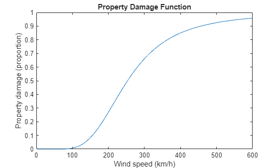
Define and Visualize Damage Function

Define a function that estimates property damage using the wind speeds of the hurricanes.

Define Damage Function

The propertyDamage helper function uses an algorithm from [4] to estimate property damage based on wind velocity and data about the property. The output of the function is the percentage of the property value that is destroyed. The inputs of the function are the wind velocity, the velocity at which the property begins to take damage, and the velocity at which half the property value is destroyed. The velocity units are km/h.

For wind velocities between 1 and 600 km/h, estimate the damage to a property asset that starts losing value at 65 km/h and loses half its value at 253 km/h. The values of vthresh and vhalf are calibration values from [3].

v = 1:600; 
vthresh = 65; 
vhalf = 253;  
damage = propertyDamage(v,vthresh,vhalf);

Plot the property damage as a function of wind speed.

figure
plot(v,damage)
xlabel("Wind speed (km/h)")
ylabel("Property damage (proportion)")
title("Property Damage Function")

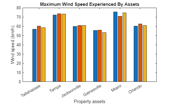
Calculate Maximum Wind Speed Experienced by Assets

The propertyDamage function assumes that the wind velocity corresponds to the location of the property asset. The windSpeedCalculator helper object and windSpeed helper function use algorithms from [6] and [5] to calculate the maximum wind speed experienced by a property over the course of a given hurricane.

• A windSpeedCalculator object stores the coordinates of the hurricane centers, the maximum wind speed values, the radius to maximum winds value, and the minimum pressure values. The hurricane data provides this information.

• The windSpeed function uses a windSpeedCalculator object, the coordinates of the property, and the distance from the property to the sea. The asset data provides this information.

Prepare to calculate the maximum wind speeds experienced by the property assets by creating a new subtable of hurricane centers for the AOI. For this subtable, include the hurricane centers that do not make landfall.

isfloridahcane = isinterior(aoi,Shape);
floridahcanes = hcanes(isfloridahcane,:);

Using the same sample hurricane as before, calculate the maximum wind speeds experienced by the property assets.

• Using the new subtable, extract the table rows for the sample hurricane.

• Create a windSpeedCalculator object from the data associated with the sample hurricane.

• Use the windSpeed function to calculate the maximum wind speed experienced by each property asset.

• Display the maximum wind speeds using a bar graph. Each bar represents a property asset. Group the bars according to city.

% Get table rows for sample hurricane
sampleind = floridahcanes.TCnumber==sampleTCnum & floridahcanes.Year==sampleYear;
samplehcane = floridahcanes(sampleind,:);

% Create wind speed calculator
wsc = windSpeedCalculator(samplehcane.Shape.Latitude,samplehcane.Shape.Longitude, ...
    samplehcane.MaximumWindSpeed,samplehcane.RadiusToMaximumWinds,samplehcane.MinimumPressure);

% Calculate maximum wind speed for each property
v = windSpeed(wsc,assets.Shape.Latitude',assets.Shape.Longitude',assets.DistanceToSea');

% Create bar graph
figure
x = ["Tallahassee","Tampa","Jacksonville","Gainesville","Miami","Orlando"];
y = [v(1:3); v(4:6); v(7:9); v(10:12); v(13:15); v(16:18)];
bar(x,y)
title("Maximum Wind Speed Experienced By Assets")
xlabel("Property assets")
ylabel("Wind speed (km/h)")

Calculate Property Losses

Calculate the property damage for each simulated year and property asset by using the windSpeedCalculator object, the windSpeed function, and the propertyDamage function. This strategy assumes that the highest wind velocity experienced by a property over the course of a year determines the property damage for the year. Note that, in practice, damage functions typically include additional information about the hazard and the property.

Initialize a table that stores the property damage for each simulated year in terms of percent loss and dollar loss. Preallocate the table elements using zero values.

years = unique(floridahcanes.Year);
numyears = numel(years);
numassets = height(assets);
floridahcanelosses = table(zeros(numyears,1),zeros(numyears,numassets),zeros(numyears,numassets), ...
    VariableNames=["Year","PercentLosses","DollarLosses"]);

Calculate the property damage for each simulated year and hurricane. Within two loops that iterate through each simulated year and hurricane ID, perform these tasks:

• Extract the table rows that correspond to the simulated year and the hurricane ID.

• If more than one data point for the hurricane ID exists, calculate the maximum wind speed experienced by each property asset.

• Calculate the property damage for each property asset.

• Add a new row to the table that includes the year, the percent losses for each property asset, and the dollar losses for each property asset. Calculate the dollar losses using the property values from the assets table.

for yearInd = 1:numyears
    year = years(yearInd);
    yearhcanes = floridahcanes(floridahcanes.Year == year,:);

    TCnums = unique(yearhcanes.TCnumber);
    v = zeros(1,numassets);
    for TCnum = TCnums'
        % Get table rows that correspond to year and ID
        hcane = yearhcanes(yearhcanes.TCnumber == TCnum,:);

        if height(hcane) > 1
            % Calculate maximum wind speed experienced by each property
            wsc = windSpeedCalculator(hcane.Shape.Latitude,hcane.Shape.Longitude, ...
                hcane.MaximumWindSpeed,hcane.RadiusToMaximumWinds,hcane.MinimumPressure);
            v2 = windSpeed(wsc,assets.Shape.Latitude',assets.Shape.Longitude',assets.DistanceToSea');
            v = max(v,v2);
        end
    end

    % Calculate property damage
    damage = propertyDamage(v,vthresh,vhalf);

    % Store results in table
    floridahcanelosses.Year(yearInd) = year;
    floridahcanelosses.PercentLosses(yearInd,:) = damage*100;
    floridahcanelosses.DollarLosses(yearInd,:) = damage.*assets.AssetValues';
end

The table of property damages only includes rows for years where hurricanes pass through the AOI. Prepare to calculate average outcomes by creating a new table that contains a row for each simulated year.

• Initialize a new table that includes a row for each simulated year. Preallocate the table elements using zero values.

• Iterate through each simulated year. If the table of property damages includes a row for the year, then copy the row to the new table. Otherwise, keep the zero values.

% Initialize new table
allyears = unique(hcanes.Year);
numallyears = numel(allyears);
hcanelosses = table(zeros(numallyears,1),zeros(numallyears,numassets),zeros(numallyears,numassets), ...
    VariableNames=["Year","PercentLosses","DollarLosses"]);

% Iterate through each year
for yearInd = 1:numel(allyears)
    year = allyears(yearInd);
    if ismember(year,years)
        hcanelosses(yearInd,:) = floridahcanelosses(floridahcanelosses.Year == year,:);
    else
        hcanelosses.Year(yearInd) = year;
    end
end

Analyze Property Losses

The table hcanelosses stores the property damage for each simulated year in terms of percent loss and dollar loss. Analyze the results by viewing the losses for a selected property and for a portfolio of all the properties.

Query Losses for Selected Property

Select a property from the assets table by specifying a row number. Display the corresponding row of the table.

propertyNum =2;
disp(assets(propertyNum,:))

            Shape                                   Name                           AdminLevel    AssetValues    DistanceToSea
    ______________________    _________________________________________________    __________    ___________    _____________

    (30.4022°N, 84.3360°W)    "3226 Flastacowo Rd, Tallahassee, FL, 32310, USA"    "address"      5.545e+05          35      

For each simulated year, query the percent and dollar losses for the property.

percentLosses = hcanelosses.PercentLosses(:,propertyNum);
dollarLosses = hcanelosses.DollarLosses(:,propertyNum);

Calculate and display the largest loss experienced by the property.

maxPercentLoss = max(percentLosses);
maxDollarLoss = max(dollarLosses);
fprintf("Largest Percent Loss: " + maxPercentLoss + "\n" + "Largest Dollar Loss: " + maxDollarLoss)

Largest Percent Loss: 8.2338
Largest Dollar Loss: 45656.2922

Calculate and display the expected loss per year by calculating the average of the losses.

meanPercentLoss = mean(percentLosses);
meanDollarLoss = mean(dollarLosses);
fprintf("Expected Percent Loss: " + meanPercentLoss + "\n" + "Expected Dollar Loss: " + meanDollarLoss)

Expected Percent Loss: 0.059618
Expected Dollar Loss: 330.5824

For risk management purposes, a more realistic metric is percentile loss. Calculate and display the dollar loss for the property at the 95th percentile.

percentile = 0.95;
percentileDollarLoss = quantile(dollarLosses,percentile);
fprintf("Dollar Loss at 95th Percentile: " + percentileDollarLoss)

Dollar Loss at 95th Percentile: 1266.2186

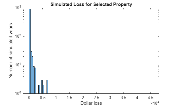
View Loss Distribution for Selected Property

View the distribution of the dollar losses by creating a histogram. Improve the visibility of the tail by changing the y-axis scale to logarithmic.

figure
histogram(dollarLosses)
title("Simulated Loss for Selected Property")
ylabel("Number of simulated years")
xlabel("Dollar loss")
yscale log

Query Losses for All Properties

Analyze the NatCat risk for a portfolio of all the property assets. For each simulated year, sum the losses for all the properties. Then, calculate the dollar losses for the entire portfolio at the 95th percentile.

yearlyTotalDollarLosses = sum(hcanelosses.DollarLosses,2);
yearlyTotalDollarPercentileLosses = quantile(yearlyTotalDollarLosses,percentile);
fprintf("Total Dollar Loss at 95th Percentile: " + yearlyTotalDollarPercentileLosses)

Total Dollar Loss at 95th Percentile: 60899.9064

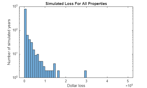
View Loss Distribution for All Properties

View the distribution of the dollar losses for the portfolio by creating a new histogram.

figure
histogram(yearlyTotalDollarLosses)
title("Simulated Loss For All Properties")
ylabel("Number of simulated years")
xlabel("Dollar loss")
yscale log

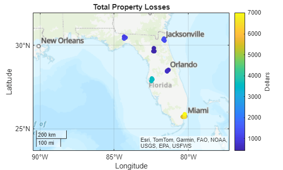
Display Total Property Losses on Map

Add a new variable to the assets table that stores the total dollar loss for each property at the 95th percentile.

TotalPercentileLosses = quantile(hcanelosses.DollarLosses,percentile)';
assets = addvars(assets,TotalPercentileLosses);

Display each property on a new map. Indicate the total dollar loss for each property asset by applying a color to the corresponding marker. Add a labeled color bar, change the geographic limits, and add a title.

figure
geobasemap topographic
geoplot(assets,ColorVariable="TotalPercentileLosses",MarkerSize=20)

c = colorbar;
c.Label.String = "Dollars";

geolimits(latlim,lonlim);
title("Total Property Losses")

Helper Functions

propertyDamage Function

The propertyDamage function estimates property damage based on the specified wind velocity and property data. From [4], the percent of the property value that is destroyed $\mathit{D}$ is:

$\mathit{D}=\frac{{\mathit{W}}^3}{1+{\mathit{W}}^3}$, where:

$$\mathit{W}=\frac{\max \left(\left[\mathit{V}-{\mathit{V}}_{\mathrm{thresh}}\right],0\right)}{{\mathit{V}}_{\mathrm{half}}-{\mathit{V}}_{\mathrm{thresh}}}$$,

and $\mathit{V}$ is the wind velocity, ${\mathit{V}}_{\mathrm{thresh}}$ is the velocity at which the property begins to take damage, and ${\mathit{V}}_{\mathrm{half}}$ is the velocity at which half of the property value is destroyed.

function D = propertyDamage(v,vthresh,vhalf)
    k = size(v,2);
    v = max(v - vthresh,zeros(1,k))./(vhalf - vthresh);
    D = (v.^3)./(1 + v.^3);
end

windSpeedCalculator Object and windSpeed Function

The windSpeedCalculator object and the windSpeed function calculate the maximum wind speed experienced by a property asset over the course of a hurricane. The object and function are attached to the example as a supporting file.

• For a given hurricane, a windSpeedCalculator object stores the coordinates of the hurricane centers, the maximum wind speed values, the radius to maximum winds value, and the minimum pressure values. The example specifies these inputs using the hurricane data from [2].

• For a given property asset, the inputs to windSpeed are a windSpeedCalculator object, the coordinates of the property, and the distance from the property to the sea. The example specifies these inputs using the asset data stored in assets.

From [6], the maximum wind velocity ${\mathit{V}}_{\mathit{i}}$ experienced by a property asset over the course of a given hurricane is:

${\mathit{V}}_{\mathit{i}}=\mathrm{GF}\left[{\mathit{V}}_{\mathit{m}}-\mathit{S}\left(1-\sin \left({\mathit{T}}_{\mathit{i}}\right)\right)\frac{{\mathit{V}}_{\mathit{h}}}{2}\right]\times {\left[{\left(\frac{{\mathit{R}}_{\mathit{m}}}{{\mathit{R}}_{\mathit{i}}}\right)}^{\mathit{B}}\exp \left(1-{\left[\frac{{\mathit{R}}_{\mathit{m}}}{{\mathit{R}}_{\mathit{i}}}\right]}^{\mathit{B}}\right)\right]}^{\frac{1}{2}}$,

where:

• $\mathit{G}=1.5$ is the gust factor, from [6].

• $\mathit{F}=0.7\left(1-\mathit{R}\right)$ is the friction parameter, from [6]. $\mathit{R}$ is a reduction factor that scales linearly as a function of distance inland. The reduction factor starts at 0.14 and scales to 0.28 at 50 km from the coast.

• $\mathit{S}=1$ is the storm asymmetry factor, from [6].

• ${\mathit{V}}_{\mathit{m}}$ is the maximum wind velocity in km/h, from the hurricane data.

• ${\mathit{T}}_{\mathit{i}}$ is the clockwise angle made by the forward direction of the hurricane and the line made by the property asset and the hurricane center. The windSpeed function calculates the forward direction of the hurricane from the hurricane data.

• ${\mathit{V}}_{\mathit{h}}$ is the forward velocity of the hurricane in km/h. The windSpeed function calculates ${\mathit{V}}_{\mathit{h}}$ from the hurricane data.

• ${\mathit{R}}_{\mathit{m}}$ is the radius to maximum winds, from the hurricane data.

• ${\mathit{R}}_{\mathit{i}}$ is the radius to the property asset in km. The windSpeed function calculates ${\mathit{R}}_{\mathit{i}}$ from the hurricane data and the asset data.

• $\mathit{B}$ is the wind profile parameter, defined by [5].

From [5], the wind profile parameter $\mathit{B}$ is $\mathit{B}=1.6\times {\mathit{B}}_{\mathit{s}}$, where:

${\mathit{B}}_{\mathit{s}}=-4.4\times {10}^{-5}{\Delta \mathit{p}}^2+0.01\Delta \mathit{p}+0.03\frac{{\partial \mathit{p}}_{\mathit{c}}}{\partial \mathit{t}}-0.014\varphi +0.15{\mathit{V}}_{\mathit{t}}^{\mathit{x}}+1$,

and:

• $\mathit{x}=0.6\times \left(1-\frac{\Delta \mathit{p}}{215}\right)$.

• $$\Delta \mathit{p}={\mathit{p}}_{\mathit{n}}-{\mathit{p}}_{\mathit{c}}$$.

• ${\mathit{p}}_{\mathit{n}}=1016$ is the normal atmospheric pressure in hPa, from [5].

• ${\mathit{p}}_{\mathit{c}}$ is the atmospheric pressure in the center of the hurricane in hPa, from the hurricane data.

• $\frac{{\partial \mathit{p}}_{\mathit{c}}}{\partial \mathit{t}}$ is the change in central pressure over time in hPa/h. The windSpeed function calculates this value from the hurricane data.

• $\varphi$ is the absolute value of the latitude of the property, from the hurricane data.

• ${\mathit{V}}_{\mathit{t}}$ is the forward velocity of the hurricane in m/s. The windSpeed function calculates ${\mathit{V}}_{\mathit{t}}$ from the hurricane data.

References

[1] Bloemendaal, Nadia, Ivan D. Haigh, Hans De Moel, Sanne Muis, Reindert J. Haarsma, and Jeroen C. J. H. Aerts. "Generation of a Global Synthetic Tropical Cyclone Hazard Dataset Using STORM." Scientific Data 7, no. 1 (February 6, 2020): 40. https://doi.org/10.1038/s41597-020-0381-2.

[2] Bloemendaal, Nadia, I.D. (Ivan) Haigh, H. (Hans) de Moel, S Muis, R.J. (Reindert) Haarsma, and J.C.J.H. (Jeroen) Aerts. "STORM IBTrACS Present Climate Synthetic Tropical Cyclone Tracks." Media types: application/vnd.google-earth.kml+xml, application/zip, text/plain. 4TU.Centre for Research Data, September 30, 2020. https://doi.org/10.4121/UUID:82C1DC0D-5485-43D8-901A-CE7F26CDA35D.

[3] Bressan, Giacomo, Anja Duranovic, Irene Monasterolo, and Stefano Battiston. “Asset-Level Climate Physical Risk Assessment and Cascading Financial Losses.” SSRN Electronic Journal, 2022. https://doi.org/10.2139/ssrn.4062275.

[4] Emanuel, Kerry. "Global Warming Effects on U.S. Hurricane Damage." Weather, Climate, and Society 3, no. 4 (October 1, 2011): 261–68. https://doi.org/10.1175/WCAS-D-11-00007.1.

[5] Holland, Greg. "A Revised Hurricane Pressure–Wind Model." Monthly Weather Review 136, no. 9 (September 1, 2008): 3432–45. https://doi.org/10.1175/2008MWR2395.1.

[6] Ishizawa, Oscar A., Juan José Miranda, and Eric Strobl. "The Impact of Hurricane Strikes on Short-Term Local Economic Activity: Evidence from Nightlight Images in the Dominican Republic." International Journal of Disaster Risk Science 10, no. 3 (September 2019): 362–70. https://doi.org/10.1007/s13753-019-00226-0.

[7] Foote, Matthew, John Hillier, Kirsten Mitchell‐Wallace, and Matthew Jones. Natural Catastrophe Risk Management and Modelling: A Practitioner's Guide. 1st ed. Wiley, 2017. https://doi.org/10.1002/9781118906057.