imbilatfilt
Bilateral filtering of images with Gaussian kernels
Syntax
Description
J = imbilatfilt(I,degreeOfSmoothing)degreeOfSmoothing is a
small value, imbilatfilt smooths neighborhoods with small
variance (uniform areas) but does not smooth neighborhoods with large variance, such
as strong edges. When the value of degreeOfSmoothing increases,
imbilatfilt smooths both uniform areas and neighborhoods with
larger variance.
J = imbilatfilt(I,degreeOfSmoothing,spatialSigma)spatialSigma, of the
spatial Gaussian smoothing kernel. Larger values of
spatialSigma increase the contribution of more distant
neighboring pixels, effectively increasing the neighborhood size.
J = imbilatfilt(___,Name=Value)
Examples
Read and display a grayscale image. Observe the horizontal striation artifact in the sky region.
I = imread('cameraman.tif');
imshow(I)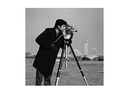
Inspect a patch of the image from the sky region. Compute the variance of the patch, which approximates the variance of the noise.
patch = imcrop(I,[170, 35, 50 50]);
imshow(patch)
patchVar = std2(patch)^2;
Filter the image using bilateral filtering. Set the degree of smoothing to be larger than the variance of the noise.
DoS = 2*patchVar;
J = imbilatfilt(I,DoS);
imshow(J)
title(['Degree of Smoothing: ',num2str(DoS)])
The striation artifact is reduced, but not eliminated. To improve the smoothing, increase the value of spatialSigma to 2 so that distant neighboring pixels contribute more to the Gaussian smoothing kernel. This effectively increases the spatial extent of the bilateral filter.
K = imbilatfilt(I,DoS,2);
imshow(K)
title(['Degree of Smoothing: ',num2str(DoS),', Spatial Sigma: 2'])
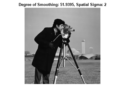
The striation artifact in the sky is successfully removed. The sharpness of strong edges such as the silhouette of the man, and textured regions such as the grass in the foreground of the image, have been preserved.
Read an RGB image.
imRGB = imread("coloredChips.png");
imshow(imRGB)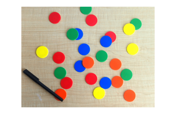
Convert the image to the L*a*b* color space, so that the bilateral filter smooths perceptually similar colors.
imLAB = rgb2lab(imRGB);
Extract a patch that contains no sharp edges. Compute the variance in the Euclidean distance from the origin, in the L*a*b* color space.
patch = imcrop(imLAB,[34,71,60,55]);
patchSq = patch.^2;
edist = sqrt(sum(patchSq,3));
patchVar = std2(edist).^2;
Filter the image in the L*a*b* color space using bilateral filtering. Set the DegreeOfSmoothing value to be higher than the variance of the patch.
DoS = 2*patchVar;
smoothedLAB = imbilatfilt(imLAB,DoS);
Convert the image back to the RGB color space, and display the smoothed image.
smoothedRBG = lab2rgb(smoothedLAB,"Out","uint8");
montage({imRGB,smoothedRBG})
title("Original Image vs. Filtered Image with Degree of Smoothing: "+num2str(DoS))
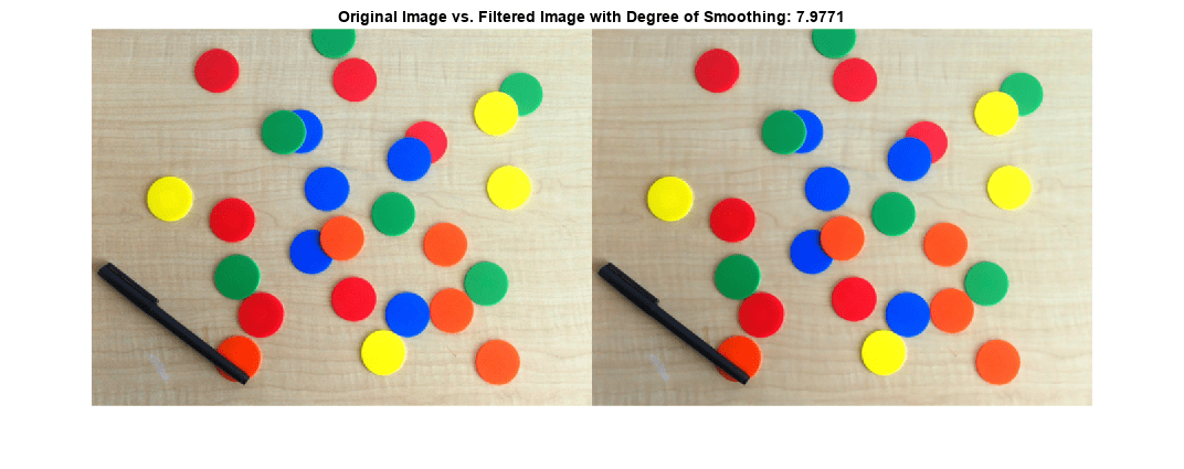
The colors of the chips and black pen appear more uniform, but the horizontal grains in the table are still visible. Increase the spatial extent of the filter so that the effective neighborhood of the filter spans the space between the horizontal grains (this distance is approximately seven pixels). Also increase the DegreeOfSmoothing to smooth these regions more aggressively.
DoS2 = 4*patchVar;
sigma = 7;
smoothedLAB2 = imbilatfilt(imLAB,DoS2,sigma);
smoothedRBG2 = lab2rgb(smoothedLAB2,"Out","uint8");
montage({imRGB,smoothedRBG2})
title("Original Image vs. Filtered Image with Degree of Smoothing: "+num2str(DoS)+ ...
    " and Spatial Sigma: "+sigma)

The color of the wooden table is more uniform with the larger neighborhood and larger degree of smoothing. The edge sharpness of the chips and pen is preserved.
Input Arguments
Name-Value Arguments
Output Arguments
Tips
The value of
degreeOfSmoothingcorresponds to the variance of the Range Gaussian kernel of the bilateral filter [1]. The Range Gaussian is applied on the Euclidean distance of a pixel value from the values of its neighbors.To smooth perceptually close colors of an RGB image, convert the image to the CIE L*a*b* space using
rgb2labbefore applying the bilateral filter. To view the results, convert the filtered image to RGB usinglab2rgb.Increasing
spatialSigmaincreasesNeighborhoodSize, which increases the filter execution time. You can specify a smallerNeighborhoodSizeto trade accuracy for faster execution time.
References
[1] Tomasi, C., and R. Manduchi. "Bilateral Filtering for Gray and Color Images". Proceedings of the 1998 IEEE® International Conference on Computer Vision. Bombay, India. Jan 1998, pp. 836–846.
Extended Capabilities
Version History
Introduced in R2018aSee Also
imdiffusefilt | imgaussfilt | imguidedfilter | imfilter | nlfilter | locallapfilt | imnlmfilt