Ground Plane Segmentation and Obstacle Detection on NVIDIA Jetson Xavier NX Embedded Platforms

This example shows how to perform ground plane segmentation of 3-D lidar data from a vehicle on NVIDIA® embedded platforms to find nearby obstacles.

The example uses ground plane segmentation and obstacle detection to illustrate:

• C++ and CUDA® code generation for the ground plane segmentation and obstacle detection algorithm by using MATLAB® Coder™ and GPU Coder™.

• Verification of the generated code on the target platform by using processor-in-the-loop (PIL) simulation.

• The performance of the application on the CPU (C++) and the GPU (CUDA).

Third-Party Prerequisites

Target Board Requirements

• NVIDIA Jetson™ Xavier™ NX Embedded platform.

• NVIDIA CUDA toolkit.

• Environment variables for the compilers and libraries. For more information, see Install and Setup Prerequisites for NVIDIA Boards.

Development Host Requirements

• NVIDIA CUDA toolkit.

• Environment variables for the compilers and libraries. For information on the supported versions of the compilers and libraries, see Third-Party Hardware. For setting up the environment variables, see Setting Up the Prerequisite Products.

Configure and Verify NVIDIA Target Platform

Connect to NVIDIA Hardware

The MATLAB Coder Support Package for NVIDIA Jetson and NVIDIA DRIVE® Platforms uses SSH connection over TCP/IP to execute commands while building and running the generated code on the Jetson platforms. Connect the target platform to the same network as the host computer.

To communicate with the NVIDIA hardware, create a live hardware connection object by using the jetson function. This example uses the device address, user name, and password settings from the most recent successful connection to the Jetson hardware.

hwobj = jetson;

Checking for CUDA availability on the Target...
Checking for 'nvcc' in the target system path...
Checking for cuDNN library availability on the Target...
Checking for TensorRT library availability on the Target...
Checking for prerequisite libraries is complete.
Gathering hardware details...
Checking for third-party library availability on the Target...
Gathering hardware details is complete.
 Board name              : NVIDIA Jetson Nano Developer Kit
 CUDA Version            : 10.2
 cuDNN Version           : 8.2
 TensorRT Version        : 8.2
 GStreamer Version       : 1.14.5
 V4L2 Version            : 1.14.2-1
 SDL Version             : 1.2
 OpenCV Version          : 4.1.1
 Available Webcams       :  
 Available GPUs          : NVIDIA Tegra X1
 Available Digital Pins  : 7  11  12  13  15  16  18  19  21  22  23  24  26  29  31  32  33  35  36  37  38  40

Configure PIL Simulation

This example uses processor-in-the-loop (PIL) simulation to test the generated C++ and CUDA code on the Jetson board. Because the input data transfer and algorithm computations consume time, change the default PIL timeout value to prevent time-out errors.

setPILTimeout(hwobj,100);

Verify GPU Environment

To verify that the compilers and libraries necessary for running this example are set up correctly, use the coder.checkGpuInstall function.

envCfg = coder.gpuEnvConfig('jetson');
envCfg.BasicCodegen = 1;
envCfg.Quiet = 1;
envCfg.HardwareObject = hwobj;
coder.checkGpuInstall(envCfg);

When the Quiet property of the coder.gpuEnvConfig object is set to true, the coder.checkGpuInstall function returns only warning or error messages.

Configure Code Generation Parameters

To generate a PIL executable that runs on the ARM® CPU of the Jetson board, create a coder.EmbeddedCodeConfig object for a static library.

cfgCpu = coder.config('lib');

Set the target language for the generated code to C++ and enable PIL execution in the code configuration object. Then, enable execution-time profiling during PIL execution. Execution-time profiling generates metrics for tasks and functions in the generated code. For more information, see Create Execution-Time Profile for Generated Code (Embedded Coder). Finally, create a coder.hardware object for the Jetson platform and assign it to the Hardware property of the code configuration object.

cfgCpu.TargetLang = 'C++';
cfgCpu.VerificationMode = 'PIL';
cfgCpu.CodeExecutionProfiling = true;
cfgCpu.Hardware = coder.hardware('NVIDIA Jetson');

Similarly, create configuration parameters for the CUDA GPU on the Jetson board by using coder.gpuConfig.

cfgGpu = coder.gpuConfig('lib');
cfgGpu.VerificationMode = 'PIL';
cfgGpu.CodeExecutionProfiling = true;
cfgGpu.Hardware = coder.hardware('NVIDIA Jetson');

segmentGroundAndObstacles Entry-Point Function

The segmentGroundAndObstacles entry-point function segments points that belong to the ground plane, the ego vehicle, and nearby obstacles from the input point cloud locations. This diagram illustrates the algorithm implemented in the entry-point function. For more information, see Ground Plane and Obstacle Detection Using Lidar (Automated Driving Toolbox).

type segmentGroundAndObstacles

function [egoPoints, groundPoints, obstaclePoints] = ...
    segmentGroundAndObstacles(ptCloudLocation)
%segmentGroundAndObstacles segments ground and nearby obstacle points from 
%the pointcloud.
%   egoPoints = segmentGroundAndObstacles(ptCloudLocation) segments the 
%   ground points and nearby obstacle points from the input argument 
%   ptCloudLocation. egoPoints are the vehicle points segmented with the 
%   help of helper function helperSegmentEgoFromLidarData. 
%   segmentGroundFromLidarData is used to segment the ground points, 
%   groundPoints. findNeighborsInRadius is used to segment the nearby 
%   obstacles, obstaclePoints.
%
%   [..., groundPoints, obstaclePoints] = segmentGroundAndObstacles(...)
%   additionally returns segmented groundPoints and obstaclePoints.

%   Copyright 2021 The MathWorks, Inc.

%#codegen

% GPU Coder pragma
coder.gpu.kernelfun;

% Create a pointCloud object for point cloud locations
ptCloud = pointCloud(ptCloudLocation);

%% Segment the Ego Vehicle
% The lidar is mounted on top of the vehicle, and the point cloud may 
% contain points belonging to the vehicle itself, such as on the roof or 
% hood. Knowing the dimensions of the vehicle, we can segment out points 
% that are closest to the vehicle.

% Create a vehicleDimensions object for storing dimensions of the vehicle.
% Typical vehicle 4.7m by 1.8m by 1.4m

vehicleDims.Length = 4.7;
vehicleDims.Width = 1.8;
vehicleDims.Height = 1.4;
vehicleDims.RearOverhang = 1.0;

% Specify the mounting location of the lidar in the vehicle coordinate 
% system. The vehicle coordinate system is centered at the center of the 
% rear-axle, on the ground, with positive X direction pointing forward, 
% positive Y towards the left, and positive Z upwards. In this example, 
% the lidar is mounted on the top center of the vehicle, parallel to the 
% ground.

mountLocation = [...
    vehicleDims.Length/2 - vehicleDims.RearOverhang, ... % x
    0, ...                                               % y
    vehicleDims.Height];                                 % z

% Segment the ego vehicle using the helper function 
% |helperSegmentEgoFromLidarData|. This function segments all points within
% the cuboid defined by the ego vehicle. 

egoPoints = helperSegmentEgoFromLidarData(ptCloudLocation, vehicleDims, mountLocation);

%% Segment Ground Plane and Nearby Obstacles
% In order to identify obstacles from the lidar data, first segment the 
% ground plane using the segmentGroundFromLidarData function to accomplish 
% this. This function segments points belonging to the ground from organized 
% lidar data.

elevationDelta = 10;
groundPoints = segmentGroundFromLidarData(ptCloud, 'ElevationAngleDelta', elevationDelta);

% Remove points belonging to the ego vehicle and the ground plane by using 
% the select function on the point cloud. Specify the 'OutputSize' as 
% 'full' to retain the organized nature of the point cloud. For CUDA code 
% generation, an optimized approach for removing the points is considered.

nonEgoGroundPoints = coder.nullcopy(egoPoints);
coder.gpu.kernel;
for iter = 1:numel(egoPoints)
    nonEgoGroundPoints(iter) = ~egoPoints(iter) & ~groundPoints(iter);
end

ptCloudSegmented = select(ptCloud, nonEgoGroundPoints, 'OutputSize', 'full');

% Next, segment nearby obstacles by looking for all points that are not 
% part of the ground or ego vehicle within some radius from the ego
% vehicle. This radius can be determined based on the range of the lidar 
% and area of interest for further processing.

sensorLocation  = [0, 0, 0]; % Sensor is at the center of the coordinate system
radius          = 40; % meters

obstaclePoints = findNeighborsInRadius(ptCloudSegmented, sensorLocation, radius);

end


function egoPoints = helperSegmentEgoFromLidarData(ptCloudLocation, vehicleDims, mountLocation)
%#codegen
%helperSegmentEgoFromLidarData segment ego vehicle points from lidar data
%   egoPoints = helperSegmentEgoFromLidarData(ptCloudLocation,vehicleDims,mountLocation)
%   segments points belonging to the ego vehicle of dimensions vehicleDims
%   from the lidar scan ptCloud. The lidar is mounted at location specified
%   by mountLocation in the vehicle coordinate system. ptCloud is a
%   pointCloud object. vehicleDimensions is a vehicleDimensions object.
%   mountLocation is a 3-element vector specifying XYZ location of the
%   lidar in the vehicle coordinate system.
%
%   This function assumes that the lidar is mounted parallel to the ground
%   plane, with positive X direction pointing ahead of the vehicle,
%   positive Y direction pointing to the left of the vehicle in a
%   right-handed system.

% GPU Coder pragma
coder.gpu.kernelfun;

% Buffer around ego vehicle 
bufferZone = [0.1, 0.1, 0.1]; % in meters

% Define ego vehicle limits in vehicle coordinates
egoXMin = -vehicleDims.RearOverhang - bufferZone(1);
egoXMax = egoXMin + vehicleDims.Length + bufferZone(1);
egoYMin = -vehicleDims.Width/2 - bufferZone(2);
egoYMax = egoYMin + vehicleDims.Width + bufferZone(2);
egoZMin = 0 - bufferZone(3);
egoZMax = egoZMin + vehicleDims.Height + bufferZone(3);

egoXLimits = [egoXMin, egoXMax];
egoYLimits = [egoYMin, egoYMax];
egoZLimits = [egoZMin, egoZMax];

% Transform to lidar coordinates
egoXLimits = egoXLimits - mountLocation(1);
egoYLimits = egoYLimits - mountLocation(2);
egoZLimits = egoZLimits - mountLocation(3);

% Use logical indexing to select points inside ego vehicle cube
egoPoints = ptCloudLocation(:,:,1) > egoXLimits(1) ...
    & ptCloudLocation(:,:,1) < egoXLimits(2) ...
    & ptCloudLocation(:,:,2) > egoYLimits(1) ...
    & ptCloudLocation(:,:,2) < egoYLimits(2) ...
    & ptCloudLocation(:,:,3) > egoZLimits(1) ...
    & ptCloudLocation(:,:,3) < egoZLimits(2);
end

Generate and Run Executables on the Target

The point cloud data from the lidar sensor is of size 32-by-1100-by-3. However, due to signal misses and noise, using an upper bound of 1100 for the second dimension may exclude some points from the point cloud data. Use the coder.typeof function to specify varriable dimensions for the second dimension.

codegenArgs = {coder.typeof(single(0),[32,1100,3],[0,1,0])};

Generate and Run C++ Executable

Generate C++ code with the CPU code configuration object cfgCpu.

codegen -config cfgCpu -args codegenArgs segmentGroundAndObstacles -report

### Connectivity configuration for function 'segmentGroundAndObstacles': 'NVIDIA Jetson'
PIL execution is using Port 17725.
PIL execution is using 100 Sec(s) for receive time-out.
Code generation successful: View report

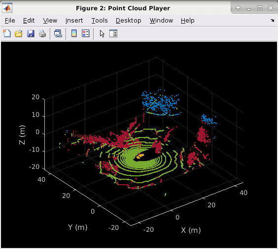
The obstacleDetectionWrapper helper function is an execution wrapper that processess the streaming lidar input data frame-by-frame, calls the PIL executable, and displays the 3-D point cloud with segmenting points that belong to the ground plane, the ego vehicle, and nearby obstacles. The lidar data used in this example was recorded using a Velodyne® HDL32E sensor mounted on a vehicle. For an explanation of the processing performed by the obstacleDetectionWrapper function, see Ground Plane and Obstacle Detection Using Lidar (Automated Driving Toolbox).

obstacleDetectionWrapper();

### Starting application: 'codegen/lib/segmentGroundAndObstacles/pil/segmentGroundAndObstacles.elf'
    To terminate execution: clear segmentGroundAndObstacles_pil
### Launching application segmentGroundAndObstacles.elf...
    Execution profiling data is available for viewing. Open Simulation Data Inspector.
    Execution profiling report will be available after termination.

Collect Execution Profile of the C++ Executable

Clear the PIL executable and collect the execution time profile by using the getCoderExecutionProfile function.

clear segmentGroundAndObstacles_pil;

Runtime log on Target:
[sudo] password for ubuntu: 
PIL execution terminated on target.
    Execution profiling report: coder.profile.show(getCoderExecutionProfile('segmentGroundAndObstacles'))

cpuExecutionProfile = getCoderExecutionProfile('segmentGroundAndObstacles');

Generate and Run CUDA Executable

Generate CUDA code with the GPU code configuration object cfgGpu.

codegen -config cfgGpu -args codegenArgs segmentGroundAndObstacles -report

### Connectivity configuration for function 'segmentGroundAndObstacles': 'NVIDIA Jetson'
PIL execution is using Port 17725.
PIL execution is using 100 Sec(s) for receive time-out.
Code generation successful: View report

To maximize the GPU performance, use the jetson_clocks.sh script on the board. For more information, see NVIDIA Xavier - Maximizing Performance (RidgeRun wiki).

ClockFileStatus = system(hwobj, 'test -f l4t_dfs.conf && echo "1" || echo "0"');
if ~str2double(ClockFileStatus)
    system(hwobj,'echo "ubuntu" | sudo -S jetson_clocks --store | printf "y"');
end
system(hwobj,'echo "ubuntu" | sudo -S jetson_clocks');

Use the obstacleDetectionWrapper helper function to process the streaming lidar input data, call the PIL executable, and display the 3-D point cloud with segmenting points that belong to the ground plane, the ego vehicle, and nearby obstacles.

obstacleDetectionWrapper();

### Starting application: 'codegen/lib/segmentGroundAndObstacles/pil/segmentGroundAndObstacles.elf'
    To terminate execution: clear segmentGroundAndObstacles_pil
### Launching application segmentGroundAndObstacles.elf...
    Execution profiling data is available for viewing. Open Simulation Data Inspector.
    Execution profiling report will be available after termination.

Collect Execution Profile of the CUDA Executable

Disable the Jetson clock settings, clear the PIL executable, and collect the execution time profile by using the getCoderExecutionProfile function.

system(hwobj,'echo "ubuntu" | sudo -S jetson_clocks --restore');
clear segmentGroundAndObstacles_pil;

Runtime log on Target:
[sudo] password for ubuntu: 
PIL execution terminated on target.
    Execution profiling report: coder.profile.show(getCoderExecutionProfile('segmentGroundAndObstacles'))

gpuExecutionProfile = getCoderExecutionProfile('segmentGroundAndObstacles');

Analysis of CPU and GPU Execution Profiles

Get the per-frame execution times of the CPU and GPU from their execution profiles by using the ExecutionTimeInSeconds property.

[~,cpuExecTimePerFrame,~] = cpuExecutionProfile.Sections.ExecutionTimeInSeconds;
[~,gpuExecTimePerFrame,~] = gpuExecutionProfile.Sections.ExecutionTimeInSeconds;

To plot the per frame execution times, use this code:

figure;
% Plot CPU execution times.
plot(cpuExecTimePerFrame(2:end)*1000,'r');
hold on;
% Plot GPU execution times.
plot(gpuExecTimePerFrame(2:end)*1000,'b');
grid on;
% Set the title, legend and labels.
title('CPU vs GPU Per-frame Execution times (in ms)');
legend('CPU Timings', 'GPU Timings');
axis([0,40,0,40]);
xlabel('Frame Number');
ylabel('Execution Time (in ms)');

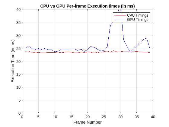
These numbers are representative. The actual values depend on your hardware capabilities.

Supporting Functions

The obstacleDetectionWrapper helper function processess the lidar data, calls the PIL executable, and visualizes the results. For an explanation of the processing performed by the obstacleDetectionWrapper function, see Ground Plane and Obstacle Detection Using Lidar (Automated Driving Toolbox).

function obstacleDetectionWrapper()
%OBSTACLEDETECTIONWRAPPER process lidar data and visualize results
%   The OBSTACLEDETECTIONWRAPPER is an execution wrapper function that
%   processess the streaming lidar input data frame-by-frame, calls the PIL
%   executable, and displays the 3-D point cloud with segmenting points
%   belonging to the ground plane, the ego vehicle, and nearby obstacles.

fileName    = 'lidarData_ConstructionRoad.pcap';
deviceModel = 'HDL32E';
veloReader = velodyneFileReader(fileName, deviceModel);

% Setup Streaming Point Cloud Display
xlimits = [-25 45];   % Limits of point cloud display, meters
ylimits = [-25 45];
zlimits = [-20 20];

% Create a pcplayer
lidarViewer = pcplayer(xlimits, ylimits, zlimits);
xlabel(lidarViewer.Axes, 'X (m)')
ylabel(lidarViewer.Axes, 'Y (m)')
zlabel(lidarViewer.Axes, 'Z (m)')

% Set the colormap for labeling the ground plane, ego vehicle, and nearby
% obstacles.
colorLabels = [...
    0      0.4470 0.7410; ... % Unlabeled points, specified as [R,G,B]
    0.4660 0.6740 0.1880; ... % Ground points
    0.9290 0.6940 0.1250; ... % Ego points
    0.6350 0.0780 0.1840];    % Obstacle points

% Define indices for each label
colors.Unlabeled = 1;
colors.Ground    = 2;
colors.Ego       = 3;
colors.Obstacle  = 4;

% Set the colormap
colormap(lidarViewer.Axes, colorLabels)

% Stop processing the frame after specified time.
stopTime = veloReader.EndTime;

i = 1;
isPlayerOpen = true;
while hasFrame(veloReader) && veloReader.CurrentTime < stopTime && isPlayerOpen

    % Grab the next lidar scan
    ptCloud = readFrame(veloReader);

    % Segment points belonging to the ego vehicle
    [egoPoints,groundPoints,obstaclePoints] = segmentGroundAndObstacles_pil(ptCloud.Location);

    i = i+1;
    closePlayer = ~hasFrame(veloReader);

    % Update lidar display
    points = struct('EgoPoints',egoPoints, 'GroundPoints',groundPoints, ...
        'ObstaclePoints',obstaclePoints);
    isPlayerOpen = helperUpdateView(lidarViewer, ptCloud, points, colors, closePlayer);
end
snapnow
end

The helperUpdateView helper function updates the streaming point cloud display with the latest point cloud and associated color labels.

function isPlayerOpen = helperUpdateView(lidarViewer,ptCloud,points,colors,closePlayer)
%HELPERUPDATEVIEW update streaming point cloud display
%   isPlayerOpen =
%   HELPERUPDATEVIEW(lidarViewer,ptCloud,points,colors,closePlayers)
%   updates the pcplayer object specified in lidarViewer with a new point
%   cloud ptCloud. Points specified in the struct points are colored
%   according to the colormap of lidarViewer using the labels specified by
%   the struct colors. closePlayer is a flag indicating whether to close
%   the lidarViewer.

if closePlayer
    hide(lidarViewer);
    isPlayerOpen = false;
    return;
end

scanSize = size(ptCloud.Location);
scanSize = scanSize(1:2);

% Initialize colormap
colormapValues = ones(scanSize, 'like', ptCloud.Location) * colors.Unlabeled;

if isfield(points, 'GroundPoints')
    colormapValues(points.GroundPoints) = colors.Ground;
end

if isfield(points, 'EgoPoints')
    colormapValues(points.EgoPoints) = colors.Ego;
end

if isfield(points, 'ObstaclePoints')
    colormapValues(points.ObstaclePoints) = colors.Obstacle;
end

% Update view
view(lidarViewer, ptCloud.Location, colormapValues)

% Check if player is open
isPlayerOpen = isOpen(lidarViewer);

end