Predict Chaotic Time-Series Using ANFIS

This example shows how to do chaotic time-series prediction using ANFIS.

Time Series Data

This example uses anfis to predict a time series generated by the following Mackey-Glass (MG) time-delay differential equation.

$x_{}^{˙} (t) = \frac{0.2 x (t - τ)}{1 + x^{10} (t - τ)} - 0.1 x (t)$

This time series is chaotic with no clearly defined period. The series does not converge or diverge, and the trajectory is highly sensitive to initial conditions. This benchmark problem is used in the neural network and fuzzy modeling research communities.

To obtain the time series value at integer points, the fourth-order Runge-Kutta method was used to find the numerical solution to the previous MG equation. It was assumed that $x (0) = 1.2$ , $τ = 17$ , and $x (t) = 0$ for $t < 0$ . The result was saved in the file mgdata.dat.

Load and plot the MG time series.

load mgdata.dat
time = mgdata(:,1);
x = mgdata(:, 2);
figure(1)
plot(time,x)
title('Mackey-Glass Chaotic Time Series')
xlabel('Time (sec)')
ylabel('x(t)')

Figure contains an axes object. The axes object with title Mackey-Glass Chaotic Time Series, xlabel Time (sec), ylabel x(t) contains an object of type line.

Preprocess Data

In time-series prediction, you use known values of the time series up to point in time, $t$ , to predict the value at some point in the future, $t + P$ . The standard method for this type of prediction is to create a mapping from $D$ sample data points, sampled every $Δ$ units in time ( $x (t - (D - 1) Δ), \dots, x (t - Δ), x (t)$ ) to a predicted future value $x = (t + P)$ . Following the conventional settings for predicting the MG time series, set $D = 4$ and $Δ = P = 6$ . For each $t$ , the input training data for anfis is a four-column vector of the following form.

$w (t) = [x (t - 19), x (t - 12), x (t - 6), x (t)]$

The output training data corresponds to the trajectory prediction.

$s (t) = x (t + 6)$

For each $t$ , ranging in values from 118 to 1117, there are 1000 input/output training samples. For this example, use the first 500 samples as training data (trnData) and the second 500 values as checking data for validation (chkData). Each row of the training and checking data arrays contains one sample point where the first four columns contain the four-dimensional input $w$ and the fifth column contains the output $s$ .

Construct the training and checking data arrays.

for t = 118:1117 
    Data(t-117,:) = [x(t-18) x(t-12) x(t-6) x(t) x(t+6)]; 
end
trnData = Data(1:500,:);
chkData = Data(501:end,:);

Build Initial Fuzzy System

Create an initial Sugeno FIS object for training using the genfis function with grid partitioning.

fis = genfis(trnData(:,1:end-1),trnData(:,end),...
    genfisOptions('GridPartition'));

The number of FIS inputs and outputs corresponds to the number of columns in the input and output training data, four and one, respectively.

By default, genfis creates two generalized bell membership functions for each of the four inputs. The initial membership functions for each variable are equally spaced and cover the whole input space.

figure
subplot(2,2,1)
plotmf(fis,'input',1)
subplot(2,2,2)
plotmf(fis,'input',2)
subplot(2,2,3)
plotmf(fis,'input',3)
subplot(2,2,4)
plotmf(fis,'input',4)

The generated FIS object contains $2^{4}$ = 16 fuzzy rules with 104 parameters (24 nonlinear parameters and 80 linear parameters). To achieve good generalization capability, it is important that the number of training data points be several times larger than the number parameters being estimated. In this case, the ratio between data and parameters is approximately five (500/104), which is a good balance between fitting parameters and training sample points.

Train ANFIS Model

To configure training options, create an anfisOptions option set, specifying the initial FIS and validation data.

options = anfisOptions('InitialFIS',fis,'ValidationData',chkData);

Train the FIS using the specified training data and options.

[fis1,error1,ss,fis2,error2] = anfis(trnData,options);

ANFIS info:
	Number of nodes: 55
	Number of linear parameters: 80
	Number of nonlinear parameters: 24
	Total number of parameters: 104
	Number of training data pairs: 500
	Number of checking data pairs: 500
	Number of fuzzy rules: 16


Start training ANFIS ...

1 	 0.00296046 	 0.00292488
2 	 0.00290346 	 0.0028684
3 	 0.00285048 	 0.00281544
4 	 0.00280117 	 0.00276566
Step size increases to 0.011000 after epoch 5.
5 	 0.00275517 	 0.00271874
6 	 0.00271214 	 0.00267438
7 	 0.00266783 	 0.00262818
8 	 0.00262626 	 0.00258435
Step size increases to 0.012100 after epoch 9.
9 	 0.00258702 	 0.00254254
10 	 0.00254972 	 0.00250247

Designated epoch number reached. ANFIS training completed at epoch 10.

Minimal training RMSE = 0.00254972
Minimal checking RMSE = 0.00250247

fis1 is the trained fuzzy inference system for the training epoch where the training error is smallest. Since you specified validation data, the fuzzy system with the minimum checking error, fis2, is also returned. The FIS with the smallest checking error shows the best generalization beyond the training data.

Plots the membership functions for the trained system.

figure
subplot(2,2,1)
plotmf(fis2,'input',1)
subplot(2,2,2)
plotmf(fis2,'input',2)
subplot(2,2,3)
plotmf(fis2,'input',3)
subplot(2,2,4)
plotmf(fis2,'input',4)

Plot Errors Curves

Plot the training and checking error signals.

figure
plot([error1 error2])
hold on
plot([error1 error2],'o')
legend('Training error','Checking error')
xlabel('Epochs')
ylabel('Root Mean Squared Error')
title('Error Curves')

Figure contains an axes object. The axes object with title Error Curves, xlabel Epochs, ylabel Root Mean Squared Error contains 4 objects of type line. One or more of the lines displays its values using only markers These objects represent Training error, Checking error.

The training error is higher than the checking error in all epochs. This phenomenon is not uncommon in ANFIS learning or nonlinear regression in general; it could indicate that additional training could produce better training results.

Compare Original and Predicted Series

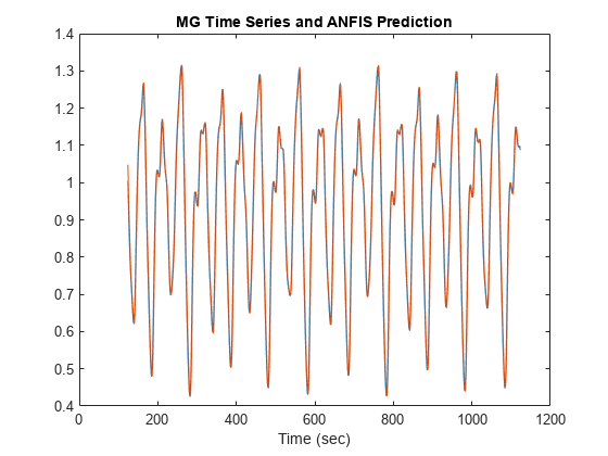
To check prediction capability of the trained system, evaluate the fuzzy system using the training and checking data, and plot the result alongside the original.

anfis_output = evalfis(fis2,[trnData(:,1:4); chkData(:,1:4)]);

figure
index = 125:1124;
plot(time(index),[x(index) anfis_output])
xlabel('Time (sec)')
title('MG Time Series and ANFIS Prediction')

Figure contains an axes object. The axes object with title MG Time Series and ANFIS Prediction, xlabel Time (sec) contains 2 objects of type line.

The predicted series is similar to the original series.

Calculate and plot the prediction error.

diff = x(index) - anfis_output;
plot(time(index),diff)
xlabel('Time (sec)')
title('Prediction Errors')

Figure contains an axes object. The axes object with title Prediction Errors, xlabel Time (sec) contains an object of type line.

The scale of the prediction error plot is about one-hundredth of the scale of the time-series plot. In this example, you trained the system for only 10 epoch. Training for additional epochs can improve the training results.