Bond Portfolio Optimization Using Portfolio Object
This example shows how to use a Portfolio object to construct an optimal portfolio of 10, 20, and 30 year treasuries that will be held for a period of one month. The workflow for the overall asset allocation process is:
Load market data — Historic daily treasury yields downloaded from FRED® are loaded.
Calculate market invariants — Daily changes in yield to maturity are chosen as invariants and assumed to be multivariate normal. Due to missing data for the 30 year bonds, an expectation maximization algorithm is used to estimate the mean and covariance of the invariants. The invariant's statistics are projected to the investment horizon.
Simulate invariants at horizon — Due to the high correlation and inherent structure in the yield curves, a principal component analysis is applied to the invariant statistics. Multivariate normal random draws are done in the PCA space. The simulations are transformed back into the invariant space using the PCA loadings.
Calculate distribution of returns at horizon — The simulated monthly changes in the yield curve are used to calculate the yield for the portfolio securities at the horizon. This requires interpolating values off of the simulated yield curves since the portfolio securities will have maturities that are one month less than 10, 20 and 30 years. Profit and loss for each scenario/security is calculated by pricing the treasuries using the simulated and interpolated yields. Simulated linear returns and their statistics are calculated from the prices.
Optimize asset allocation — Using a
Portfolioobject, mean-variance optimization is performed on the treasury returns statistics to calculate optimal portfolio weights for ten points along the efficient frontier. The investor preference is to choose the portfolio that is closest to the mean value of possible Sharpe ratios.
Load Market Data
Load the historic yield-to-maturity data for the series: DGS6MO, DGS1, DGS2, DGS3, DGS5, DGS7, DGS10, DGS20, DGS30 for the dates: Sep 1, 2000 to Sep 1, 2010 obtained from: https://fred.stlouisfed.org/categories/115.
Note: Data is downloaded using Datafeed Toolbox™ using commands like: >> conn = fred; >> data = fetch(conn,'DGS10','9/1/2000','9/1/2010'); results have been aggregated and stored in a binary HistoricalYTMData.mat file for convenience.
histData = load('HistoricalYTMData.mat');
% Time to maturity for each series
tsYTMMats = histData.tsYTMMats;
% Dates that rates were observed
tsYTMObsDates = histData.tsYTMObsDates;
% Observed rates
tsYTMRates = histData.tsYTMRates;

% Visualize the yield surface.
[X,Y] = meshgrid(tsYTMMats,tsYTMObsDates);
surf(X,Y,tsYTMRates,EdgeColor='none')
xlabel('Time to Maturity')
ylabel('Observation Dates')
zlabel('Yield to Maturity')
title('Historic Yield Surface')

Calculate Market Invariants
For market invariants, use the standard: daily changes in yield to maturity for each series. You can estimate their statistical distribution to be multivariate normal. IID analysis on each invariant series produces decent results - more so in the "independent" factor than "identical". A more thorough modeling using more complex distributions and/or time series models is beyond the scope of this example. What will need to be accounted for is the estimation of distribution parameters in the presence of missing data. The 30 year bonds were discontinued for a period between Feb 2002 and Feb 2006, so there are no yields for this time period.
% Invariants are assumed to be daily changes in YTM rates.
tsYTMRateDeltas = diff(tsYTMRates);
About 1/3 of the 30 year rates (column 9) are missing from the original data set. Rather than throw out all these observations, an expectation maximization routine ecmnmle is used to estimate the mean and covariance of the invariants. The default option (NaN skip for initial estimates) is used.
[tsInvMu,tsInvCov] = ecmnmle(tsYTMRateDeltas);
Calculate standard deviations and correlations using cov2corr.
[tsInvStd,tsInvCorr] = cov2corr(tsInvCov);
The investment horizon is 1 month (21 business days between 9/1/2010 and 10/1/2010). Since the invariants are summable and the means and variances of normal distributions are normal, you can project the invariants to the investment horizon as follows:
hrznInvMu = 21*tsInvMu';
hrznInvCov = 21*tsInvCov;
[hrznInvStd,hrznInvCor] = cov2corr(hrznInvCov);
The market invariants projected to the horizon have the following statistics:
disp('Mean:');Mean:
disp(hrznInvMu);
   1.0e-03 *

   -0.5149   -0.4981   -0.4696   -0.4418   -0.3788   -0.3268   -0.2604   -0.2184   -0.1603
disp('Standard Deviation:');Standard Deviation:
disp(hrznInvStd);
0.0023 0.0024 0.0030 0.0032 0.0033 0.0032 0.0030 0.0027 0.0026
disp('Correlation:');Correlation:
disp(hrznInvCor);
    1.0000    0.8553    0.5952    0.5629    0.4980    0.4467    0.4028    0.3338    0.3088
    0.8553    1.0000    0.8282    0.7901    0.7246    0.6685    0.6175    0.5349    0.4973
    0.5952    0.8282    1.0000    0.9653    0.9114    0.8589    0.8055    0.7102    0.6642
    0.5629    0.7901    0.9653    1.0000    0.9519    0.9106    0.8664    0.7789    0.7361
    0.4980    0.7246    0.9114    0.9519    1.0000    0.9725    0.9438    0.8728    0.8322
    0.4467    0.6685    0.8589    0.9106    0.9725    1.0000    0.9730    0.9218    0.8863
    0.4028    0.6175    0.8055    0.8664    0.9438    0.9730    1.0000    0.9562    0.9267
    0.3338    0.5349    0.7102    0.7789    0.8728    0.9218    0.9562    1.0000    0.9758
    0.3088    0.4973    0.6642    0.7361    0.8322    0.8863    0.9267    0.9758    1.0000
Simulate Market Invariants at Horizon
The high correlation is not ideal for simulation of the distribution of invariants at the horizon (and ultimately security prices). Use a principal component decomposition to extract orthogonal invariants. This could also be used for dimension reduction, however since the number of invariants is still relatively small, retain all nine components for more accurate reconstruction. However, missing values in the market data prevents you from estimating directly off of the time series data. Instead, this can be done directly off of the covariance matrix
% Perform PCA decomposition using the invariants' covariance.
[pcaFactorCoeff,pcaFactorVar,pcaFactorExp] = pcacov(hrznInvCov);

% Keep all components of pca decompositon.
numFactors = 9;

% Create a PCA factor covariance matrix.
pcaFactorCov = corr2cov(sqrt(pcaFactorVar),eye(numFactors));

% Define the number of simulations (random draws).
numSim = 10000;

% Fix the random seed for reproducible results.
stream = RandStream('mrg32k3a');
RandStream.setGlobalStream(stream);

% Take random draws from a multivariate normal distribution with zero mean
% and diagonal covariance.
pcaFactorSims = mvnrnd(zeros(numFactors,1),pcaFactorCov,numSim);

% Transform to horizon invariants and calculate the statistics.
hrznInvSims = pcaFactorSims*pcaFactorCoeff + repmat(hrznInvMu,numSim,1);
hrznInvSimsMu = mean(hrznInvSims);
hrznInvSimsCov = cov(hrznInvSims);
[hrznInvSimsStd,hrznInvSimsCor] = cov2corr(hrznInvSimsCov);
The simulated invariants have very similar statistics to the original invariants:
disp('Mean:');Mean:
disp(hrznInvSimsMu);
   1.0e-03 *

   -0.5222   -0.5118   -0.4964   -0.4132   -0.3255   -0.3365   -0.2508   -0.2171   -0.1636
disp('Standard Deviation:');Standard Deviation:
disp(hrznInvSimsStd);
0.0016 0.0047 0.0046 0.0025 0.0040 0.0017 0.0007 0.0005 0.0004
disp('Correlation:');Correlation:
disp(hrznInvSimsCor);
    1.0000    0.8903    0.7458   -0.4746   -0.4971    0.4885   -0.2353   -0.0971    0.1523
    0.8903    1.0000    0.9463   -0.7155   -0.6787    0.5164   -0.2238   -0.0889    0.2198
    0.7458    0.9463    1.0000   -0.8578   -0.7610    0.4659   -0.1890   -0.0824    0.2631
   -0.4746   -0.7155   -0.8578    1.0000    0.9093   -0.4999    0.2378    0.1084   -0.2972
   -0.4971   -0.6787   -0.7610    0.9093    1.0000   -0.7159    0.3061    0.1118   -0.2976
    0.4885    0.5164    0.4659   -0.4999   -0.7159    1.0000   -0.5360   -0.1542    0.1327
   -0.2353   -0.2238   -0.1890    0.2378    0.3061   -0.5360    1.0000    0.3176   -0.1108
   -0.0971   -0.0889   -0.0824    0.1084    0.1118   -0.1542    0.3176    1.0000    0.0093
    0.1523    0.2198    0.2631   -0.2972   -0.2976    0.1327   -0.1108    0.0093    1.0000
Calculate Distribution of Security Returns at Horizon
The portfolio will consist of 10, 20, and 30 year maturity treasuries. For simplicity, assume that these are new issues on the settlement date and are priced at market value inferred from the current yield curve. Profit and loss distributions are calculated by pricing each security along each simulated yield at the horizon and subtracting the purchase price. The horizon prices require nonstandard time to maturity yields. These are calculated using cubic spline interpolation. Simulated linear returns are their statistics that are calculated from the profit and loss scenarios.
% Define the purchase and investment horizon dates.
settleDate = datetime(2010,9,1);
hrznDate = datetime(2010,10,1);

% Define the maturity dates for new issue treasuries purchased on the
% settle date.
treasuryMaturities = [datetime(2020,9,1) , datetime(2030,9,1) , datetime(2040,9,1)];

% Select the observed yields for the securities of interest on the
% settle date.
treasuryYTMAtSettle = tsYTMRates(end,7:9);

% Initialize arrays for later use.
treasuryYTMAtHorizonSim = zeros(numSim,3);
treasuryPricesAtSettle = zeros(1,3);
treasuryPricesAtHorizonSim = zeros(numSim,3);

% Use actual/actual day count basis with annualized yields.
basis = 8;
Price the treasuries at settle date with bndprice using the known yield to maturity. For simplicity, assume that none of these securities include coupon payments. Although the prices may not be accurate, the overall structure/relationships between values is preserved for the asset allocation process.
for j=1:3
    treasuryPricesAtSettle(j) = bndprice(treasuryYTMAtSettle(j),0,settleDate, ...
                                         treasuryMaturities(j),'basis',basis);
end
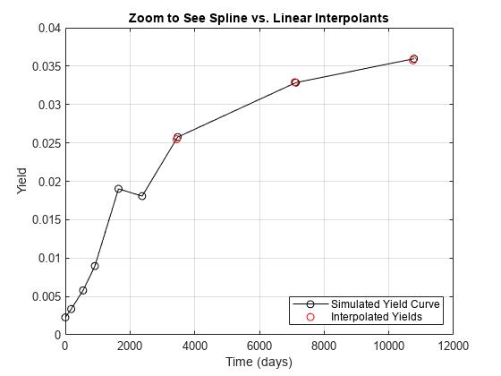
To price the treasuries at the horizon, you need to know yield to maturity at 9 years 11 months, 19 years 11 months, and 29 years 11 months for each simulation. You can approximate these using cubic spline interpolation using interp1.
% Transform the simulated invariants to YTM at the horizon.
hrznYTMRatesSims = repmat(tsYTMRates(end,:),numSim,1) + hrznInvSims;

hrznYTMMaturities = [datetime(2011,4,1),datetime(2011,10,1),datetime(2012,10,1),datetime(2013,10,1),datetime(2015,10,1),datetime(2017,10,1),datetime(2020,10,1),datetime(2030,10,1),datetime(2040,10,1)];

% Convert the dates to numeric serial dates.
x = datenum(hrznYTMMaturities);
xi = datenum(treasuryMaturities);

% For numerical accuracy, shift the x values to start at zero.
minDate = min(x);
x = x - minDate;
xi = xi - minDate;
For each simulation and maturity approximate yield near 10,20, and 30 year nodes. Note that the effects of a spline fit vs. linear fit have a significant effect on the resulting ideal allocation. This is due to significant under-estimation of yield when using a linear fit for points just short of the known nodes.
for i=1:numSim
	treasuryYTMAtHorizonSim(i,:) = interp1(x,hrznYTMRatesSims(i,:),xi,'spline');
end

% Visualize a simulated yield curve with interpolation.
figure;
plot(x,hrznYTMRatesSims(1,:),'k-o',xi,treasuryYTMAtHorizonSim(1,:),'ro');
xlabel('Time (days)');
ylabel('Yield');
legend({'Simulated Yield Curve','Interpolated Yields'},'location','se');
grid on;
title('Zoom to See Spline vs. Linear Interpolants');
Price the treasuries at the horizon for each simulated yield to maturity. Note that the same assumptions are being made here as in the previous call to bndprice.
basis = 8*ones(numSim,1);
for j=1:3
    treasuryPricesAtHorizonSim(:,j) = bndprice(treasuryYTMAtHorizonSim(:,j),0, ...
                                               hrznDate,treasuryMaturities(j),'basis',basis);
end

% Calculate the distribution of linear returns.
treasuryReturns = ( treasuryPricesAtHorizonSim - repmat(treasuryPricesAtSettle,numSim,1) )./repmat(treasuryPricesAtSettle,numSim,1);

% Calculate the returns statistics.
retsMean = mean(treasuryReturns);
retsCov  = cov(treasuryReturns);
[retsStd,retsCor] = cov2corr(retsCov);

% Visualize the results for the 30 year treasury.
figure
histogram(treasuryReturns(:,1),100,Normalization='pdf',EdgeColor='none')
hold on
histogram(treasuryReturns(:,2),100,Normalization='pdf',EdgeColor='none')
histogram(treasuryReturns(:,3),100,Normalization='pdf',EdgeColor='none')
hold off
title('Distribution of Returns for 10, 20, 30 Year Treasuries');
grid on
legend({'10 year','20 year','30 year'});

Optimize Asset Allocation Using Portfolio Object
Asset allocation is optimized using a Portfolio object. Ten optimal portfolios (NumPorts) are calculated using estimateFrontier and their Sharpe ratios are calculated. The optimal portfolio, based on investor preference, is chosen to be the one that is closest to the maximum value of the Sharpe ratio.
Create a Portfolio object using Portfolio. You can use setAssetMoments to set moments (mean and covariance) of asset returns for the Portfolio object and setDefaultConstraints to set up the portfolio constraints with nonnegative weights that sum to 1.
% Create a portfolio object.
p = Portfolio;
p = setAssetMoments(p,retsMean,retsCov);
p = setDefaultConstraints(p)
p =
Portfolio with properties:
BuyCost: []
SellCost: []
RiskFreeRate: []
AssetMean: [3×1 double]
AssetCovar: [3×3 double]
TrackingError: []
TrackingPort: []
Turnover: []
BuyTurnover: []
SellTurnover: []
Name: []
NumAssets: 3
AssetList: []
InitPort: []
AInequality: []
bInequality: []
AEquality: []
bEquality: []
LowerBound: [3×1 double]
UpperBound: []
LowerBudget: 1
UpperBudget: 1
GroupMatrix: []
LowerGroup: []
UpperGroup: []
GroupA: []
GroupB: []
LowerRatio: []
UpperRatio: []
MinNumAssets: []
MaxNumAssets: []
ConditionalBudgetThreshold: []
ConditionalUpperBudget: []
BoundType: [3×1 categorical]
Calculate ten points along the projection of the efficient frontier using estimateFrontier and estimatePortMoments to estimate moments of portfolio returns for the Portfolio object.
NumPorts = 10;
PortWts = estimateFrontier(p,NumPorts);
[PortRisk, PortReturn] = estimatePortMoments(p,PortWts);

% Visualize the portfolio.
figure;
subplot(2,1,1)
plot(PortRisk,PortReturn,'k-o');
xlabel('Portfolio Risk');
ylabel('Portfolio Return');
title('Efficient Frontier Projection');
legend('Optimal Portfolios','location','se');
grid on;

subplot(2,1,2)
bar(PortWts','stacked');
xlabel('Portfolio Number');
ylabel('Portfolio Weights');
title('Percentage Invested in Each Treasury');
legend({'10 year','20 year','30 year'});

Use estimateMaxSharpeRatio to estimate efficient portfolio that maximizes Sharpe ratio for the Portfolio object.
investorPortfolioWts = estimateMaxSharpeRatio(p);
The investor percentage allocation in 10, 20, and 30 year treasuries is:
disp(investorPortfolioWts);
    0.6078
    0.1374
    0.2548
See Also
tbilldisc2yield | tbillprice | tbillrepo | tbillval01 | tbillyield | tbillyield2disc | Portfolio | setDefaultConstraints
Topics
- Pricing and Computing Yields for Fixed-Income Securities
- Computing Treasury Bill Price and Yield
- Term Structure of Interest Rates
- Sensitivity of Bond Prices to Interest Rates
- Bond Portfolio for Hedging Duration and Convexity
- Term Structure Analysis and Interest-Rate Swaps
- Creating the Portfolio Object
- Common Operations on the Portfolio Object
- Setting Up an Initial or Current Portfolio
- Asset Allocation Case Study
- Portfolio Optimization Examples Using Financial Toolbox
- Treasury Bills Defined