filter

Filter disturbances through vector error-correction (VEC) model

Syntax

Y = filter(Mdl,Z)

[Y,E] = filter(Mdl,Z)

Tbl2 = filter(Mdl,Tbl1,Presample=Presample)

[___] = filter(___,Name,Value)

Description

Y = filter(Mdl,Z) returns the numeric array Y containing the multivariate response series, which results from filtering the underlying input numeric array Z containing the multivariate disturbance series. The series in Z are associated with the model innovations process through the fully specified VEC(p – 1) model Mdl.

[Y,E] = filter(Mdl,Z) returns the numeric array containing the multivariate model innovations series E.

Tbl2 = filter(Mdl,Tbl1,Presample=Presample) returns the table or timetable Tbl2 containing the multivariate response series, which results from filtering the underlying multivariate disturbance series in the input table or timetable Tbl1. filter initializes the response series using the required table or timetable of presample data in Presample. Variables in Tbl1 are associated with the model innovations process through Mdl. (since R2022b)

filter selects the variables in Mdl.SeriesNames or all variables in Tbl1. To select different disturbance variables in Tbl1 to filter through the model, use the DisturbanceVariables name-value argument. filter selects the same variables for Presample by default, but you can select different variables by using the PresampleResponseVariables name-value argument.

[___] = filter(___,Name,Value) specifies options using one or more name-value arguments in addition to any of the input argument combinations in previous syntaxes. filter returns the output argument combination for the corresponding input arguments. For example, filter(Mdl,Z,Y0=PS,X=Exo) filters the numeric array of disturbances Z through the VEC(p – 1) model Mdl, and specifies the numeric array of presample response data PS and the numeric matrix of exogenous predictor data Exo for the model regression component.

Examples

Filter Numeric Matrix of Disturbances Through VEC Model

Consider a VEC model for the following seven macroeconomic series. Then, fit the model to the data and filter disturbances through the fitted model. Supply the disturbances as a numeric matrix.

• Gross domestic product (GDP)

• GDP implicit price deflator

• Paid compensation of employees

• Nonfarm business sector hours of all persons

• Effective federal funds rate

• Personal consumption expenditures

• Gross private domestic investment

Suppose that a cointegrating rank of 4 and one short-run term are appropriate, that is, consider a VEC(1) model.

Load the Data_USEconVECModel data set.

load Data_USEconVECModel

For more information on the data set and variables, enter Description at the command line.

Determine whether the data needs to be preprocessed by plotting the series on separate plots.

figure
tiledlayout(2,2)
nexttile
plot(FRED.Time,FRED.GDP)
title("Gross Domestic Product")
ylabel("Index")
xlabel("Date")
nexttile
plot(FRED.Time,FRED.GDPDEF)
title("GDP Deflator")
ylabel("Index")
xlabel("Date")
nexttile
plot(FRED.Time,FRED.COE)
title("Paid Compensation of Employees")
ylabel("Billions of $")
xlabel("Date")
nexttile
plot(FRED.Time,FRED.HOANBS)
title("Nonfarm Business Sector Hours")
ylabel("Index")
xlabel("Date")

figure
tiledlayout(2,2)
nexttile
plot(FRED.Time,FRED.FEDFUNDS)
title("Federal Funds Rate")
ylabel("Percent")
xlabel("Date")
nexttile
plot(FRED.Time,FRED.PCEC)
title("Consumption Expenditures")
ylabel("Billions of $")
xlabel("Date")
nexttile
plot(FRED.Time,FRED.GPDI)
title("Gross Private Domestic Investment")
ylabel("Billions of $")
xlabel("Date")

Stabilize all series, except the federal funds rate, by applying the log transform. Scale the resulting series by 100 so that all series are on the same scale.

FRED.GDP = 100*log(FRED.GDP);      
FRED.GDPDEF = 100*log(FRED.GDPDEF);
FRED.COE = 100*log(FRED.COE);       
FRED.HOANBS = 100*log(FRED.HOANBS); 
FRED.PCEC = 100*log(FRED.PCEC);     
FRED.GPDI = 100*log(FRED.GPDI);

Create a VEC(1) model using the shorthand syntax. Specify the variable names.

Mdl = vecm(7,4,1);
Mdl.SeriesNames = FRED.Properties.VariableNames

Mdl = 
  vecm with properties:

             Description: "7-Dimensional Rank = 4 VEC(1) Model with Linear Time Trend"
             SeriesNames: "GDP"  "GDPDEF"  "COE"  ... and 4 more
               NumSeries: 7
                    Rank: 4
                       P: 2
                Constant: [7×1 vector of NaNs]
              Adjustment: [7×4 matrix of NaNs]
           Cointegration: [7×4 matrix of NaNs]
                  Impact: [7×7 matrix of NaNs]
   CointegrationConstant: [4×1 vector of NaNs]
      CointegrationTrend: [4×1 vector of NaNs]
                ShortRun: {7×7 matrix of NaNs} at lag [1]
                   Trend: [7×1 vector of NaNs]
                    Beta: [7×0 matrix]
              Covariance: [7×7 matrix of NaNs]

Mdl is a vecm model object. All properties containing NaN values correspond to parameters to be estimated given data.

Estimate the model using the entire data set and the default options. By default, estimate uses the first p = 2 observations as presample data.

EstMdl = estimate(Mdl,FRED.Variables)

EstMdl = 
  vecm with properties:

             Description: "7-Dimensional Rank = 4 VEC(1) Model"
             SeriesNames: "GDP"  "GDPDEF"  "COE"  ... and 4 more
               NumSeries: 7
                    Rank: 4
                       P: 2
                Constant: [14.1329 8.77841 -7.20359 ... and 4 more]'
              Adjustment: [7×4 matrix]
           Cointegration: [7×4 matrix]
                  Impact: [7×7 matrix]
   CointegrationConstant: [-28.6082 -109.555 77.0912 ... and 1 more]'
      CointegrationTrend: [4×1 vector of zeros]
                ShortRun: {7×7 matrix} at lag [1]
                   Trend: [7×1 vector of zeros]
                    Beta: [7×0 matrix]
              Covariance: [7×7 matrix]

EstMdl is an estimated vecm model object. It is fully specified because all parameters have known values. By default, estimate imposes the constraints of the H1 Johansen VEC model form by removing the cointegrating trend and linear trend terms from the model. Parameter exclusion from estimation is equivalent to imposing equality constraints to zero.

Generate a numobs-by-7 series of random Gaussian distributed values, where numobs is the number of observations in the data minus p.

numobs = size(FRED,1) - Mdl.P;
rng(1) % For reproducibility
Z = randn(numobs,Mdl.NumSeries);

To simulate responses, filter the disturbances through the estimated model. Specify the first p = 2 observations as presample data.

Y = filter(EstMdl,Z,Y0=FRED{1:2,:});

Y is a 238-by-7 matrix of simulated responses. Columns correspond to the variable names in EstMdl.SeriesNames.

Plot the simulated and true responses.

figure
tiledlayout(2,2)
nexttile
plot(FRED.Time(3:end),[FRED.GDP(3:end) Y(:,1)])
title("Gross Domestic Product")
ylabel("Index (scaled, log)")
xlabel("Date")
legend("Simulation","True","Location","Best")
nexttile
plot(FRED.Time(3:end),[FRED.GDPDEF(3:end) Y(:,2)])
title("GDP Deflator")
ylabel("Index (scaled, log)")
xlabel("Date")
legend("Simulation","True","Location","Best")
nexttile
plot(FRED.Time(3:end),[FRED.COE(3:end) Y(:,3)])
title("Paid Compensation of Employees")
ylabel("Billions of $ (scaled, log)")
xlabel("Date")
legend("Simulation","True","Location","Best")
nexttile
plot(FRED.Time(3:end),[FRED.HOANBS(3:end) Y(:,4)])
title("Nonfarm Business Sector Hours")
ylabel("Index (scaled, log)")
xlabel("Date")
legend("Simulation","True","Location","Best")

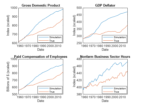
figure
tiledlayout(2,2)
nexttile
plot(FRED.Time(3:end),[FRED.FEDFUNDS(3:end) Y(:,5)])
title("Federal Funds Rate")
ylabel("Percent")
xlabel("Date")
nexttile
plot(FRED.Time(3:end),[FRED.PCEC(3:end) Y(:,6)])
title("Consumption Expenditures")
ylabel("Billions of $ (scaled, log)")
xlabel("Date")
nexttile
plot(FRED.Time(3:end),[FRED.GPDI(3:end) Y(:,7)])
title("Gross Private Domestic Investment")
ylabel("Billions of $ (scaled, log)")
xlabel("Date")

Filter Multiple Disturbance Paths

Consider this VEC(1) model for three hypothetical response series.

$$\begin{array}{rcl}\Delta y_t& =& c+A{B}^{\prime }{y}_{t-1}+{\Phi }_1\Delta y_{t-1}+{\epsilon }_t\\ & =& \\ & =& \left[\begin{array}{c}-1\\ -3\\ -30\end{array}\right]+\left[\begin{array}{cc}-0.3& 0.3\\ -0.2& 0.1\\ -1& 0\end{array}\right]\left[\begin{array}{ccc}0.1& -0.2& 0.2\\ -0.7& 0.5& 0.2\end{array}\right]y_{t-1}+\left[\begin{array}{ccc}0& 0.1& 0.2\\ 0.2& -0.2& 0\\ 0.7& -0.2& 0.3\end{array}\right]\Delta y_{t-1}+{\epsilon }_t.\end{array}$$

The innovations are multivariate Gaussian with a mean of 0 and the covariance matrix

$$\Sigma =\left[\begin{array}{ccc}1.3& 0.4& 1.6\\ 0.4& 0.6& 0.7\\ 1.6& 0.7& 5\end{array}\right].$$

Create variables for the parameter values.

Adjustment = [-0.3 0.3; -0.2 0.1; -1 0];
Cointegration = [0.1 -0.7; -0.2 0.5; 0.2 0.2];
ShortRun = {[0. 0.1 0.2; 0.2 -0.2 0; 0.7 -0.2 0.3]};
Constant = [-1; -3; -30];
Trend = [0; 0; 0];
Covariance = [1.3 0.4 1.6; 0.4 0.6 0.7; 1.6 0.7 5];

Create a vecm model object representing the VEC(1) model using the appropriate name-value pair arguments.

Mdl = vecm('Adjustment',Adjustment,'Cointegration',Cointegration,...
    'Constant',Constant,'ShortRun',ShortRun,'Trend',Trend,...
    'Covariance',Covariance)

Mdl = 
  vecm with properties:

             Description: "3-Dimensional Rank = 2 VEC(1) Model"
             SeriesNames: "Y1"  "Y2"  "Y3" 
               NumSeries: 3
                    Rank: 2
                       P: 2
                Constant: [-1 -3 -30]'
              Adjustment: [3×2 matrix]
           Cointegration: [3×2 matrix]
                  Impact: [3×3 matrix]
   CointegrationConstant: [2×1 vector of NaNs]
      CointegrationTrend: [2×1 vector of NaNs]
                ShortRun: {3×3 matrix} at lag [1]
                   Trend: [3×1 vector of zeros]
                    Beta: [3×0 matrix]
              Covariance: [3×3 matrix]

Mdl is, effectively, a fully specified vecm model object. That is, the cointegration constant and linear trend are unknown. However, they are not needed for simulating observations or forecasting, given that the overall constant and trend parameters are known.

Generate 1000 paths of 100 observations from a 3-D Gaussian distribution. numobs is the number of observations in the data without any missing values.

numobs = 100;
numpaths = 1000;
rng(1);
Z = randn(numobs,Mdl.NumSeries,numpaths);

Filter the disturbances through the estimated model. Return the innovations (scaled disturbances).

[Y,E] = filter(Mdl,Z);

Y and E are 100-by-3-by-1000 matrices of filtered responses and scaled disturbances, respectively.

For each time point, compute the mean vector of the filtered responses among all paths.

MeanFilt = mean(Y,3);

MeanFilt is a 100-by-3 matrix containing the average of the filtered responses at each time point.

Plot the filtered responses and their averages.

figure;
for j = 1:Mdl.NumSeries
    subplot(2,2,j)
    plot(squeeze(Y(:,j,:)),'Color',[0.8,0.8,0.8])
    title(Mdl.SeriesNames{j});
    hold on
    plot(MeanFilt(:,j));
    xlabel('Time index')
    hold off
end

Filter Timetable of Disturbances Through VEC Model

Since R2022b

Fit a VEC(1) model to seven macroeconomic series. Then, simulate responses by filtering multiple random paths of Gaussian distributed disturbances through the estimated model. Supply the disturbances in a timetable. This example is based on Fit VEC(1) Model to Matrix of Response Data.

Load and Preprocess Data

Load the Data_USEconVECModel data set.

load Data_USEconVECModel
head(FRED)

       Time         GDP     GDPDEF     COE     HOANBS    FEDFUNDS    PCEC     GPDI
    ___________    _____    ______    _____    ______    ________    _____    ____

    31-Mar-1957    470.6    16.485    260.6    54.756      2.96      282.3    77.7
    30-Jun-1957    472.8    16.601    262.5    54.639         3      284.6    77.9
    30-Sep-1957    480.3    16.701    265.1    54.375      3.47      289.2    79.3
    31-Dec-1957    475.7    16.711    263.7    53.249      2.98      290.8      71
    31-Mar-1958    468.4    16.892    260.2    52.043       1.2      290.3    66.7
    30-Jun-1958    472.8     16.94    259.9    51.297      0.93      293.2    65.1
    30-Sep-1958    486.7    17.043    267.7    51.908      1.76      298.3      72
    31-Dec-1958    500.4    17.123    272.7    52.683      2.42      302.2      80

Stabilize all series, except the federal funds rate, by applying the log transform. Scale the resulting series by 100 so that all series are on the same scale.

FRED.GDP = 100*log(FRED.GDP);      
FRED.GDPDEF = 100*log(FRED.GDPDEF);
FRED.COE = 100*log(FRED.COE);       
FRED.HOANBS = 100*log(FRED.HOANBS); 
FRED.PCEC = 100*log(FRED.PCEC);
FRED.GPDI = 100*log(FRED.GPDI);
numobs = height(FRED)

numobs = 
240

Prepare Timetable for Estimation

When you plan to supply a timetable directly to estimate, you must ensure it has all the following characteristics:

• All selected response variables are numeric and do not contain any missing values.

• The timestamps in the Time variable are regular, and they are ascending or descending.

Remove all missing values from the table.

DTT = rmmissing(FRED);
numobs = height(DTT)

numobs = 
240

DTT does not contain any missing values.

Determine whether the sampling timestamps have a regular frequency and are sorted.

areTimestampsRegular = isregular(DTT,"quarters")

areTimestampsRegular = logical
   0

areTimestampsSorted = issorted(DTT.Time)

areTimestampsSorted = logical
   1

areTimestampsRegular = 0 indicates that the timestamps of DTT are irregular. areTimestampsSorted = 1 indicates that the timestamps are sorted. Macroeconomic series in this example are timestamped at the end of the month. This quality induces an irregularly measured series.

Remedy the time irregularity by shifting all dates to the first day of the quarter.

dt = DTT.Time;
dt = dateshift(dt,"start","quarter");
DTT.Time = dt;
areTimestampsRegular = isregular(DTT,"quarters")

areTimestampsRegular = logical
   1

DTT is regular with respect to time.

Fit Model to Data

Create a VEC(1) model using the shorthand syntax. Specify the variable names.

Mdl = vecm(7,4,1);
Mdl.SeriesNames = string(FRED.Properties.VariableNames);

Estimate the model. Pass the entire timetable DTT. By default, estimate selects the response variables in Mdl.SeriesNames to fit to the model. Alternatively, you can use the ResponseVariables name-value argument.

EstMdl = estimate(Mdl,DTT);

Simulate Paths of Disturbances

Generate a numobs-by-numseries-by-numpaths array of independent random Gaussian distributed values, where numobs is the number of observations in the data, numseries the number of response series 7, and numpaths is 100. Add the matrices of simulated paths into the data set DTT.

rng(1) % For reproducibility
numobs = height(DTT);
numseries = EstMdl.NumSeries;
numpaths = 100;

Z = mvnrnd(zeros(numseries,1),eye(numseries),numobs*numpaths);
Z = reshape(Z,numobs,numseries,numpaths);

for j = 1:numseries
    DTT = addvars(DTT,squeeze(Z(:,j,:)), ...
        NewVariableNames="Z_" + EstMdl.SeriesNames{j});
end

head(DTT)

       Time         GDP      GDPDEF     COE      HOANBS    FEDFUNDS     PCEC      GPDI        Z_GDP          Z_GDPDEF         Z_COE          Z_HOANBS       Z_FEDFUNDS        Z_PCEC          Z_GPDI   
    ___________    ______    ______    ______    ______    ________    ______    ______    ____________    ____________    ____________    ____________    ____________    ____________    ____________

    01-Jan-1957     615.4    280.25     556.3    400.29      2.96       564.3    435.29    1×100 double    1×100 double    1×100 double    1×100 double    1×100 double    1×100 double    1×100 double
    01-Apr-1957    615.87    280.95    557.03    400.07         3      565.11    435.54    1×100 double    1×100 double    1×100 double    1×100 double    1×100 double    1×100 double    1×100 double
    01-Jul-1957    617.44    281.55    558.01    399.59      3.47      566.71    437.32    1×100 double    1×100 double    1×100 double    1×100 double    1×100 double    1×100 double    1×100 double
    01-Oct-1957    616.48    281.61    557.48     397.5      2.98      567.26    426.27    1×100 double    1×100 double    1×100 double    1×100 double    1×100 double    1×100 double    1×100 double
    01-Jan-1958    614.93    282.68    556.15    395.21       1.2      567.09    420.02    1×100 double    1×100 double    1×100 double    1×100 double    1×100 double    1×100 double    1×100 double
    01-Apr-1958    615.87    282.97    556.03    393.76      0.93      568.09    417.59    1×100 double    1×100 double    1×100 double    1×100 double    1×100 double    1×100 double    1×100 double
    01-Jul-1958    618.76    283.57    558.99    394.95      1.76      569.81    427.67    1×100 double    1×100 double    1×100 double    1×100 double    1×100 double    1×100 double    1×100 double
    01-Oct-1958    621.54    284.04    560.84    396.43      2.42      571.11     438.2    1×100 double    1×100 double    1×100 double    1×100 double    1×100 double    1×100 double    1×100 double

Filter Disturbances Through Model

When you filter disturbances by using a timetable, filter requires a presample. Split the timetable into presample and in-sample data sets. The presample data is the initial EstMdl.P observations, and the in-sample data set contains the remaining observations.

Presample = DTT(1:EstMdl.P,:);
InSample = DTT((EstMdl.P + 1):end,:);

Simulate response paths by filtering the in-sample disturbances through the estimated model. Specify the variable names of the disturbance series, the presample data, and the response variable names in the presample.

dnames = string(DTT.Properties.VariableNames);
idx = startsWith(dnames,"Z_");
dnames = dnames(idx);

Tbl2 = filter(EstMdl,InSample,DisturbanceVariables=dnames, ...
    Presample=Presample,PresampleResponseVariables=EstMdl.SeriesNames);
size(Tbl2)

ans = 1×2

   238    28

head(Tbl2)

       Time         GDP      GDPDEF     COE      HOANBS    FEDFUNDS     PCEC      GPDI        Z_GDP          Z_GDPDEF         Z_COE          Z_HOANBS       Z_FEDFUNDS        Z_PCEC          Z_GPDI       GDP_Responses    GDPDEF_Responses    COE_Responses    HOANBS_Responses    FEDFUNDS_Responses    PCEC_Responses    GPDI_Responses    GDP_Innovations    GDPDEF_Innovations    COE_Innovations    HOANBS_Innovations    FEDFUNDS_Innovations    PCEC_Innovations    GPDI_Innovations
    ___________    ______    ______    ______    ______    ________    ______    ______    ____________    ____________    ____________    ____________    ____________    ____________    ____________    _____________    ________________    _____________    ________________    __________________    ______________    ______________    _______________    __________________    _______________    __________________    ____________________    ________________    ________________

    01-Jul-1957    617.44    281.55    558.01    399.59      3.47      566.71    437.32    1×100 double    1×100 double    1×100 double    1×100 double    1×100 double    1×100 double    1×100 double    1×100 double       1×100 double      1×100 double       1×100 double         1×100 double        1×100 double      1×100 double      1×100 double         1×100 double        1×100 double         1×100 double           1×100 double          1×100 double        1×100 double  
    01-Oct-1957    616.48    281.61    557.48     397.5      2.98      567.26    426.27    1×100 double    1×100 double    1×100 double    1×100 double    1×100 double    1×100 double    1×100 double    1×100 double       1×100 double      1×100 double       1×100 double         1×100 double        1×100 double      1×100 double      1×100 double         1×100 double        1×100 double         1×100 double           1×100 double          1×100 double        1×100 double  
    01-Jan-1958    614.93    282.68    556.15    395.21       1.2      567.09    420.02    1×100 double    1×100 double    1×100 double    1×100 double    1×100 double    1×100 double    1×100 double    1×100 double       1×100 double      1×100 double       1×100 double         1×100 double        1×100 double      1×100 double      1×100 double         1×100 double        1×100 double         1×100 double           1×100 double          1×100 double        1×100 double  
    01-Apr-1958    615.87    282.97    556.03    393.76      0.93      568.09    417.59    1×100 double    1×100 double    1×100 double    1×100 double    1×100 double    1×100 double    1×100 double    1×100 double       1×100 double      1×100 double       1×100 double         1×100 double        1×100 double      1×100 double      1×100 double         1×100 double        1×100 double         1×100 double           1×100 double          1×100 double        1×100 double  
    01-Jul-1958    618.76    283.57    558.99    394.95      1.76      569.81    427.67    1×100 double    1×100 double    1×100 double    1×100 double    1×100 double    1×100 double    1×100 double    1×100 double       1×100 double      1×100 double       1×100 double         1×100 double        1×100 double      1×100 double      1×100 double         1×100 double        1×100 double         1×100 double           1×100 double          1×100 double        1×100 double  
    01-Oct-1958    621.54    284.04    560.84    396.43      2.42      571.11     438.2    1×100 double    1×100 double    1×100 double    1×100 double    1×100 double    1×100 double    1×100 double    1×100 double       1×100 double      1×100 double       1×100 double         1×100 double        1×100 double      1×100 double      1×100 double         1×100 double        1×100 double         1×100 double           1×100 double          1×100 double        1×100 double  
    01-Jan-1959    623.66    284.31    563.55    398.35       2.8      573.62    442.12    1×100 double    1×100 double    1×100 double    1×100 double    1×100 double    1×100 double    1×100 double    1×100 double       1×100 double      1×100 double       1×100 double         1×100 double        1×100 double      1×100 double      1×100 double         1×100 double        1×100 double         1×100 double           1×100 double          1×100 double        1×100 double  
    01-Apr-1959    626.19    284.46    565.91    400.24      3.39      575.54    449.31    1×100 double    1×100 double    1×100 double    1×100 double    1×100 double    1×100 double    1×100 double    1×100 double       1×100 double      1×100 double       1×100 double         1×100 double        1×100 double      1×100 double      1×100 double         1×100 double        1×100 double         1×100 double           1×100 double          1×100 double        1×100 double  

Tbl2 is a 238-by-2 matrix of in-sample data, paths of simulated disturbances, paths of filtered responses (variables names appended with _Responses, and paths of innovations (variables with name appended with _Innovations).

rnames = string(Tbl2.Properties.VariableNames);
idx = endsWith(rnames,"_Responses");
rnames = rnames(idx);

figure
tiledlayout(2,2)
for j = 1:4
    nexttile
    p1 = plot(Tbl2.Time,Tbl2{:,rnames(j)},Color=[0.5 0.5 0.5]);
    hold on
    p2 = plot(Tbl2.Time,Tbl2{:,Mdl.SeriesNames(j)},LineWidth=2);
    title(Mdl.SeriesNames(j))
    xlabel("Date")
    legend([p1(1) p2],["Simulated" "Observed"])
end

figure
tiledlayout(2,2)
for j = 5:7
    nexttile
    p1 = plot(Tbl2.Time,Tbl2{:,rnames(j)},Color=[0.5 0.5 0.5]);
    hold on
    p2 = plot(Tbl2.Time,Tbl2{:,Mdl.SeriesNames(j)},LineWidth=2);
    title(Mdl.SeriesNames(j))
    xlabel("Date")
    legend([p1(1) p2],["Simulated" "Observed"])
end

Input Arguments

Mdl — VEC model

vecm model object

VEC model, specified as a vecm model object created by vecm or estimate. Mdl must be fully specified.

Z — Underlying multivariate disturbance series

numeric matrix | numeric array

Underlying multivariate disturbance series z_t associated with the model innovations process ε_t, specified as a numobs-by-numseries numeric matrix or a numobs-by-numseries-by-numpaths numeric array.

numobs is the sample size. numseries is the number of disturbance series (Mdl.NumSeries). numpaths is the number of disturbance paths.

Rows correspond to sampling times, and the last row contains the latest set of disturbances.

Columns correspond to individual disturbance series for response variables.

Pages correspond to separate, independent paths. For a numeric matrix, Z is a single numseries-dimensional path of disturbance series. For a 3-D array, each page of Z represents a separate numseries-dimensional path. Among all pages, disturbances in corresponding rows occur at the same time.

The Scale name-value argument specifies whether to scale the disturbances before filter filters them through Mdl. For more details, see Scale.

Data Types: double

Tbl1 — Time series data

table | timetable

Since R2022b

Time series data containing observed disturbance variables z_t, associated with the model innovations process ε_t, or predictor variables x_t, specified as a table or timetable with numvars variables and numobs rows. You can optionally select numseries disturbance variables or numpreds predictor variables by using the DisturbanceVariables or PredictorVariables name-value arguments, respectively.

Each selected disturbance variable is a numobs-by-numpaths numeric matrix, and each predictor variable is a numeric vector. Each row is an observation, and measurements in each row occur simultaneously.

Each path (column) of a disturbance variable is independent of all others, but path j of all presample and in-sample variables correspond, for j = 1,…,numpaths. Each selected predictor variable contains one path, which filter applies to all paths.

If Tbl1 is a timetable, it must represent a sample with a regular datetime time step (see isregular), and the datetime vector Tbl1.Time must be ascending or descending.

If Tbl1 is a table, the last row contains the latest observation.

The Scale name-value argument specifies whether to scale the disturbances before filter filters them through Mdl. For more details, see Scale.

Presample — Presample data

table | timetable

Since R2022b

Presample data that provides initial values for the model Mdl, specified as a table or timetable, the same type as Tbl1, with numprevars variables and numpreobs rows. Presample is required when you supply a table or timetable of data Tbl1.

Each row is a presample observation, and measurements in each row, among all paths, occur simultaneously. numpreobs must be at least Mdl.P. If you supply more rows than necessary, filter uses the latest Mdl.P observations only.

Each variable is a numpreobs-by-numprepaths numeric matrix. Variables correspond to the response series associated with the respective disturbance in Tbl1. To control presample variable selection, see the optional PresampleResponseVariables name-value argument.

For each variable, columns are separate, independent paths.

• If variables are vectors, filter applies them to each path in Tbl1 to produce the filtered responses in Tbl2. Therefore, all paths of filtered responses derive from common initial conditions.

• Otherwise, for each variable Vark and each path j, filter applies Presample.Vark(:,j) to produce Tbl2.Vark(:,j). Variables must have at least numpaths columns, and filter uses only the first numpaths columns.

If Presample is a timetable, all the following conditions must be true:

• Presample must represent a sample with a regular datetime time step (see isregular).

• The inputs Tbl1 and Presample must be consistent in time such that Presample immediately precedes Tbl1 with respect to the sampling frequency and order.

• The datetime vector of sample timestamps Presample.Time must be ascending or descending.

If Presample is a table, the last row contains the latest presample observation.

Name-Value Arguments

Specify optional pairs of arguments as Name1=Value1,...,NameN=ValueN, where Name is the argument name and Value is the corresponding value. Name-value arguments must appear after other arguments, but the order of the pairs does not matter.

Before R2021a, use commas to separate each name and value, and enclose Name in quotes.

Example: filter(Mdl,Z,Y0=PS,X=Exo) filters the numeric array of disturbances Z through the VEC(p – 1) model Mdl, and specifies the numeric array of presample response data PS and the numeric matrix of exogenous predictor data Exo for the model regression component.

DisturbanceVariables — Variables to select from Tbl1 to treat as disturbance variables z_t

string vector | cell vector of character vectors | vector of integers | logical vector

Since R2022b

Variables to select from Tbl1 to treat as disturbance variables z_t, specified as one of the following data types:

• String vector or cell vector of character vectors containing numseries variable names in Tbl1.Properties.VariableNames

• A length numseries vector of unique indices (integers) of variables to select from Tbl1.Properties.VariableNames

• A length numvars logical vector, where DisturbanceVariables(j) = true selects variable j from Tbl1.Properties.VariableNames, and sum(DisturbanceVariables) is numseries

The selected variables must be numeric vectors (single path) or matrices (columns represent multiple independent paths) of the same width, and cannot contain missing values (NaN).

If the number of variables in Tbl1 matches Mdl.NumSeries, the default specifies all variables in Tbl1. If the number of variables in Tbl1 exceeds Mdl.NumSeries, the default matches variables in Tbl1 to names in Mdl.SeriesNames.

Example: DisturbanceVariables=["GDP" "CPI"]

Example: DisturbanceVariables=[true false true false] or DisturbanceVariable=[1 3] selects the first and third table variables as the disturbance variables.

Data Types: double | logical | char | cell | string

Y0 — Presample responses

numeric matrix | numeric array

Presample responses that provide initial values for the model Mdl, specified as a numpreobs-by-numseries numeric matrix or a numpreobs-by-numseries-by-numprepaths numeric array. Use Y0 only when you supply a numeric array of disturbance data Z.

numpreobs is the number of presample observations. numprepaths is the number of presample response paths.

Each row is a presample observation, and measurements in each row, among all pages, occur simultaneously. The last row contains the latest presample observation. Y0 must have at least Mdl.P rows. If you supply more rows than necessary, filter uses the latest Mdl.P observations only.

Each column corresponds to the response series associated with the respective disturbance in Z.

Pages correspond to separate, independent paths.

• If Y0 is a matrix, filter applies it to each path (page) to produce the filtered responses Y. Therefore, all paths in Y derive from common initial conditions.

• Otherwise, filter applies Y0(:,:,j) to produce Y(:,:,j). Y0 must have at least numpaths pages, and filter uses only the first numpaths pages.

By default, filter sets any necessary presample observations.

• For stationary VAR processes without regression components, filter uses the unconditional mean $$\mu ={\Phi }^{-1}(L)c.$$

• For nonstationary processes or models containing a regression component, filter sets presample observations to an array composed of zeros.

Data Types: double

PresampleResponseVariables — Variables to select from Presample to use for presample response data

string vector | cell vector of character vectors | vector of integers | logical vector

Since R2022b

Variables to select from Presample to use for presample data, specified as one of the following data types:

• String vector or cell vector of character vectors containing numseries variable names in Presample.Properties.VariableNames

• A length numseries vector of unique indices (integers) of variables to select from Presample.Properties.VariableNames

• A length numvars logical vector, where PresampleResponseVariables(j) = true selects variable j from Presample.Properties.VariableNames, and sum(PresampleResponseVariables) is numseries

The selected variables must be numeric vectors (single path) or matrices (columns represent multiple independent paths) of the same width, and cannot contain missing values (NaN).

PresampleResponseNames does not need to contain the same names as in Tbl1; filter uses the data in selected variable PresampleResponseVariables(j) as a presample for the response variable corresponding to DisturbanceVariables(j).

The default specifies the same response variables as those selected from Tbl1 (see DisturbanceVariables).

Example: PresampleResponseVariables=["GDP" "CPI"]

Example: PresampleResponseVariables=[true false true false] or PresampleResponseVariable=[1 3] selects the first and third table variables for presample data.

Data Types: double | logical | char | cell | string

X — Predictor data x_t

numeric matrix

Predictor data x_t for the regression component in the model, specified as a numeric matrix containing numpreds columns. Use X only when you supply a numeric array of disturbance data Z.

numpreds is the number of predictor variables (size(Mdl.Beta,2)).

Each row corresponds to an observation, and measurements in each row occur simultaneously. The last row contains the latest observation. X must have at least as many observations as Z. If you supply more rows than necessary, filter uses only the latest observations. filter does not use the regression component in the presample period.

Each column is an individual predictor variable. All predictor variables are present in the regression component of each response equation.

filter applies X to each path (page) in Z; that is, X represents one path of observed predictors.

By default, filter excludes the regression component, regardless of its presence in Mdl.

Data Types: double

PredictorVariables — Variables to select from Tbl1 to treat as exogenous predictor variables x_t

string vector | cell vector of character vectors | vector of integers | logical vector

Since R2022b

Variables to select from Tbl1 to treat as exogenous predictor variables x_t, specified as one of the following data types:

• String vector or cell vector of character vectors containing numpreds variable names in Tbl1.Properties.VariableNames

• A length numpreds vector of unique indices (integers) of variables to select from Tbl1.Properties.VariableNames

• A length numvars logical vector, where PredictorVariables(j) = true selects variable j from Tbl1.Properties.VariableNames, and sum(PredictorVariables) is numpreds

The selected variables must be numeric vectors and cannot contain missing values (NaN).

By default, filter excludes the regression component, regardless of its presence in Mdl.

Example: PredictorVariables=["M1SL" "TB3MS" "UNRATE"]

Example: PredictorVariables=[true false true false] or PredictorVariable=[1 3] selects the first and third table variables to supply the predictor data.

Data Types: double | logical | char | cell | string

Scale — Flag indicating whether to scale disturbances

true (default) | false

Flag indicating whether to scale disturbances by the lower triangular Cholesky factor of the model covariance matrix, specified as a value in this table. In the table:

• Z is the input array of disturbance data Z or the specified disturbance variables in the input Tbl1.

• E is the output array of innovations E or the innovation variables in the output Tbl2.

Value	Description
true	E(:,:,j) = L*Z(:,:,j), where L = chol(Mdl.Covariance,"lower")
false	No scale, E(:,:,j) = Z(:,:,j)

For each page j = 1,...,numpaths, filter filters the numobs-by-numseries matrix of innovations E(:,:,j) through the VAR(p) model Mdl using the specified scale.

Example: Scale=false

Data Types: logical

Note

• NaN values in Z, Y0, and X indicate missing values. filter removes missing values from the data by list-wise deletion.

  1. If Z is a 3-D array, then filter horizontally concatenates the pages of Z to form a numobs-by-numpaths*numseries matrix.

  2. If a regression component is present, then filter horizontally concatenates X to Z to form a numobs-by-(numpaths*numseries + numpreds) matrix. filter assumes that the last rows of each series occur at the same time.

  3. filter removes any row that contains at least one NaN from the concatenated data.

  4. filter applies steps 1 and 3 to the presample paths in Y0.

  This process ensures that the filtered responses and innovations of each path are the same size and are based on the same observation times. In the case of missing observations, the results obtained from multiple paths of Z can differ from the results obtained from each path individually.

  This data reduction reduces the effective sample size.

• filter issues an error when any table or timetable input contains missing values.

Output Arguments

Y — Filtered multivariate response series y_t

numeric matrix | numeric array

Filtered multivariate response series y_t, returned as a numobs-by-numseries numeric matrix or a numobs-by-numseries-by-numpaths numeric array. Y represents the continuation of the presample responses in Y0.

filter returns Y only when you supply the input Z.

E — Multivariate model innovation series ε_t

numeric matrix | numeric array

Multivariate model innovations series ε_t, returned as a numobs-by-numseries numeric matrix or a numobs-by-numseries-by-numpaths numeric array. For details on the value of E, see Scale.

filter returns E only when you supply the input Z.

Tbl2 — Multivariate filtered response and innovation series

table | timetable

Since R2022b

Multivariate filtered response y_t and innovation series ε_t, returned as a table or timetable, the same data type as Tbl1. filter returns Tbl2 only when you supply the input Tbl1.

Tbl2 contains the following variables:

• The filtered response variables y_t. Each filtered response variable is a numobs-by-numpaths numeric matrix, with rows representing observations and columns representing independent paths, each corresponding to the input observations and paths in Tbl1. filter names the filtered response for disturbance variable DisturbanceJ in Tbl1 DisturbanceJ_Responses. For example, if one of the selected disturbance variables in Tbl1 to filter is GDP, Tbl2 contains a variable for the corresponding filtered responses with the name GDP_Responses.

• The innovation variables ε_t. Each innovation variable is a numobs-by-numpaths numeric matrix, with rows representing observations and columns representing independent paths, each corresponding to the input observations and paths in Tbl1. filter names the innovation variable for disturbance variable DisturbanceJ in Tbl1 DisturbanceJ_Innovations. For example, if one of the selected disturbance variables in Tbl1 to filter is GDP, Tbl2 contains a variable for the corresponding innovations with the name GDP_Innovations.

• All variables Tbl1.

If Tbl1 is a timetable, Tbl1 and Tbl2 have the same row order, either ascending or descending.

Algorithms

• filter computes Y and E using this process for each page j in Z.

  1. If Scale is true, then E(:,:,j) = L*Z(:,:,j), where L = chol(Mdl.Covariance,'lower'). Otherwise, E(:,:,j) = Z(:,:,j). Set e_t = E(:,:,j).

  2. Y(:,:,j) is y_t in this system of equations.

     $$\Delta y_t={\widehat{\Phi }}^{-1}(L)\left(\widehat{c}+\widehat{d}t+\widehat{A}\widehat{B}\prime y_{t-1}+\widehat{\beta }{x}_t+e_t\right).$$

     For variable definitions, see Vector Error-Correction Model.

• filter generalizes simulate. Both functions filter a disturbance series through a model to produce responses and innovations. However, whereas simulate generates a series of mean-zero, unit-variance, independent Gaussian disturbances Z to form innovations E = L*Z, filter enables you to supply disturbances from any distribution.

• filter uses this process to determine the time origin t₀ of models that include linear time trends.

  • If you do not specify Y0, then t₀ = 0.

  • Otherwise, filter sets t₀ to size(Y0,1) – Mdl.P. Therefore, the times in the trend component are t = t₀ + 1, t₀ + 2,..., t₀ + numobs, where numobs is the effective sample size (size(Y,1) after filter removes missing values). This convention is consistent with the default behavior of model estimation in which estimate removes the first Mdl.P responses, reducing the effective sample size. Although filter explicitly uses the first Mdl.P presample responses in Y0 to initialize the model, the total number of observations in Y0 and Y (excluding missing values) determines t₀.

References

[1] Hamilton, James D. Time Series Analysis. Princeton, NJ: Princeton University Press, 1994.

[2] Johansen, S. Likelihood-Based Inference in Cointegrated Vector Autoregressive Models. Oxford: Oxford University Press, 1995.

[3] Juselius, K. The Cointegrated VAR Model. Oxford: Oxford University Press, 2006.

[4] Lütkepohl, H. New Introduction to Multiple Time Series Analysis. Berlin: Springer, 2005.

Version History

Introduced in R2017b

R2022b: filter accepts input data in tables and timetables, and return results in tables and timetables

In addition to accepting input data in numeric arrays, filter accepts input data in tables and timetables. filter chooses default series on which to operate, but you can use the following name-value arguments to select variables.

• DisturbanceVariables specifies the disturbance series names in the input data to filter through the model.

• Presample specifies the input table or regular timetable of presample response data.

• PresampleResponseVariables specifies the response series names from Presample.

• PredictorVariables specifies the predictor series names in the input data for a model regression component.