simulate
Monte Carlo simulation of state-space models
Description
[ simulates
one sample path of observations (Y,X] =
simulate(Mdl,numObs)Y) and states
(X) from a fully specified, state-space model (Mdl).
The software simulates numObs observations and
states per sample path.
[ returns
simulated responses and states with additional options specified by
one or more Y,X] =
simulate(Mdl,numObs,Name,Value)Name,Value pair arguments.
For example, specify the number of paths or model parameter values.
Examples
Suppose that a latent process is an AR(1) model. The state equation is
where is Gaussian with mean 0 and standard deviation 1.
Generate a random series of 100 observations from , assuming that the series starts at 1.5.
T = 100;
ARMdl = arima('AR',0.5,'Constant',0,'Variance',1);
x0 = 1.5;
rng(1); % For reproducibility
x = simulate(ARMdl,T,'Y0',x0);
Suppose further that the latent process is subject to additive measurement error. The observation equation is
where is Gaussian with mean 0 and standard deviation 0.75. Together, the latent process and observation equations compose a state-space model.
Use the random latent state process (x) and the observation equation to generate observations.
y = x + 0.75*randn(T,1);
Specify the four coefficient matrices.
A = 0.5;
B = 1;
C = 1;
D = 0.75;
Specify the state-space model using the coefficient matrices.
Mdl = ssm(A,B,C,D)
Mdl =
State-space model type: ssm

State vector length: 1
Observation vector length: 1
State disturbance vector length: 1
Observation innovation vector length: 1
Sample size supported by model: Unlimited

State variables: x1, x2,...
State disturbances: u1, u2,...
Observation series: y1, y2,...
Observation innovations: e1, e2,...

State equation:
x1(t) = (0.50)x1(t-1) + u1(t)

Observation equation:
y1(t) = x1(t) + (0.75)e1(t)

Initial state distribution:

Initial state means
 x1
  0

Initial state covariance matrix
     x1
 x1  1.33

State types
     x1
 Stationary
Mdl is an ssm model. Verify that the model is correctly specified using the display in the Command Window. The software infers that the state process is stationary. Subsequently, the software sets the initial state mean and covariance to the mean and variance of the stationary distribution of an AR(1) model.
Simulate one path each of states and observations. Specify that the paths span 100 periods.
[simY,simX] = simulate(Mdl,100);
simY is a 100-by-1 vector of simulated responses. simX is a 100-by-1 vector of simulated states.
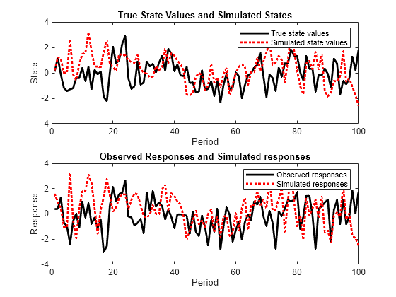
Plot the true state values with the simulated states. Also, plot the observed responses with the simulated responses.
figure
subplot(2,1,1)
plot(1:T,x,'-k',1:T,simX,':r','LineWidth',2)
title({'True State Values and Simulated States'})
xlabel('Period')
ylabel('State')
legend({'True state values','Simulated state values'})
subplot(2,1,2)
plot(1:T,y,'-k',1:T,simY,':r','LineWidth',2)
title({'Observed Responses and Simulated responses'})
xlabel('Period')
ylabel('Response')
legend({'Observed responses','Simulated responses'})

By default, simulate simulates one path for each state and observation in the state-space model. To conduct a Monte Carlo study, specify to simulate a large number of paths.
To generate variates from a state-space model, specify values for all unknown parameters.
Explicitly create this state-space model.
where and are independent Gaussian random variables with mean 0 and variance 1. Suppose that the initial state mean and variance are 1, and that the state is a stationary process.
A = NaN;
B = NaN;
C = 1;
D = NaN;
mean0 = 1;
cov0 = 1;
stateType = 0;

Mdl = ssm(A,B,C,D,'Mean0',mean0,'Cov0',cov0,'StateType',stateType);
Simulate 100 responses from Mdl. Specify that the autoregressive coefficient is 0.75, the state disturbance standard deviation is 0.5, and the observation innovation standard deviation is 0.25.
params = [0.75 0.5 0.25];
y = simulate(Mdl,100,'Params',params);

figure;
plot(y);
title 'Simulated Responses';
xlabel 'Period';

The software searches for NaN values column-wise following the order A, B, C, D, Mean0, and Cov0. The order of the elements in params should correspond to this search.
Suppose that the relationship between the change in the unemployment rate () and the nominal gross national product (nGNP) growth rate () can be expressed in the following, state-space model form.
where:
is the change in the unemployment rate at time t.
is a dummy state for the MA(1) effect on .
is the nGNP growth rate at time t.
is a dummy state for the MA(1) effect on .
is the observed change in the unemployment rate.
is the observed nGNP growth rate.
and are Gaussian series of state disturbances having mean 0 and standard deviation 1.
is the Gaussian series of observation innovations having mean 0 and standard deviation .
is the Gaussian series of observation innovations having mean 0 and standard deviation .
Load the Nelson-Plosser data set, which contains the unemployment rate and nGNP series, among other things.
load Data_NelsonPlosserPreprocess the data by taking the natural logarithm of the nGNP series, and the first difference of each. Also, remove the starting NaN values from each series.
isNaN = any(ismissing(DataTable),2);       % Flag periods containing NaNs
gnpn = DataTable.GNPN(~isNaN);
u = DataTable.UR(~isNaN);
T = size(gnpn,1);                          % Sample size
y = zeros(T-1,2);                          % Preallocate
y(:,1) = diff(u);
y(:,2) = diff(log(gnpn));
This example proceeds using series without NaN values. However, using the Kalman filter framework, the software can accommodate series containing missing values.
To determine how well the model forecasts observations, remove the last 10 observations for comparison.
numPeriods = 10;                   % Forecast horizon
isY = y(1:end-numPeriods,:);       % In-sample observations
oosY = y(end-numPeriods+1:end,:);  % Out-of-sample observations
Specify the coefficient matrices.
A = [NaN NaN NaN 0; 0 0 0 0; NaN 0 NaN NaN; 0 0 0 0];
B = [1 0;1 0 ; 0 1; 0 1];
C = [1 0 0 0; 0 0 1 0];
D = [NaN 0; 0 NaN];
Specify the state-space model using ssm. Verify that the model specification is consistent with the state-space model.
Mdl = ssm(A,B,C,D)
Mdl =
State-space model type: ssm

State vector length: 4
Observation vector length: 2
State disturbance vector length: 2
Observation innovation vector length: 2
Sample size supported by model: Unlimited
Unknown parameters for estimation: 8

State variables: x1, x2,...
State disturbances: u1, u2,...
Observation series: y1, y2,...
Observation innovations: e1, e2,...
Unknown parameters: c1, c2,...

State equations:
x1(t) = (c1)x1(t-1) + (c3)x2(t-1) + (c4)x3(t-1) + u1(t)
x2(t) = u1(t)
x3(t) = (c2)x1(t-1) + (c5)x3(t-1) + (c6)x4(t-1) + u2(t)
x4(t) = u2(t)

Observation equations:
y1(t) = x1(t) + (c7)e1(t)
y2(t) = x3(t) + (c8)e2(t)

Initial state distribution:

Initial state means are not specified.
Initial state covariance matrix is not specified.
State types are not specified.
Estimate the model parameters, and use a random set of initial parameter values for optimization. Restrict the estimate of and to all positive, real numbers using the 'lb' name-value pair argument. For numerical stability, specify the Hessian when the software computes the parameter covariance matrix, using the 'CovMethod' name-value pair argument.
rng(1);
params0 = rand(8,1);
[EstMdl,estParams] = estimate(Mdl,isY,params0,...
    'lb',[-Inf -Inf -Inf -Inf -Inf -Inf 0 0],'CovMethod','hessian');
Method: Maximum likelihood (fmincon)
Sample size: 51
Logarithmic  likelihood:      -170.92
Akaike   info criterion:       357.84
Bayesian info criterion:      373.295
      |     Coeff       Std Err    t Stat     Prob
----------------------------------------------------
 c(1) |  0.06750       0.16548     0.40791  0.68334
 c(2) | -0.01372       0.05887    -0.23302  0.81575
 c(3) |  2.71201       0.27039    10.03006   0
 c(4) |  0.83816       2.84586     0.29452  0.76836
 c(5) |  0.06274       2.83470     0.02213  0.98234
 c(6) |  0.05196       2.56873     0.02023  0.98386
 c(7) |  0.00272       2.40765     0.00113  0.99910
 c(8) |  0.00016       0.13942     0.00113  0.99910
      |
      |   Final State   Std Dev     t Stat    Prob
 x(1) | -0.00000       0.00272    -0.00033  0.99973
 x(2) |  0.12237       0.92954     0.13164  0.89527
 x(3) |  0.04049       0.00016   256.71119   0
 x(4) |  0.01183       0.00016    72.50757   0
EstMdl is an ssm model, and you can access its properties using dot notation.
Filter the estimated, state-space model, and extract the filtered states and their variances from the final period.
[~,~,Output] = filter(EstMdl,isY);
Modify the estimated, state-space model so that the initial state means and covariances are the filtered states and their covariances of the final period. This sets up simulation over the forecast horizon.
EstMdl1 = EstMdl;
EstMdl1.Mean0 = Output(end).FilteredStates;
EstMdl1.Cov0 = Output(end).FilteredStatesCov;
Simulate 5e5 paths of observations from the fitted, state-space model EstMdl. Specify to simulate observations for each period.
numPaths = 5e5;
SimY = simulate(EstMdl1,10,'NumPaths',numPaths);
SimY is a 10-by- 2-by- numPaths array containing the simulated observations. The rows of SimY correspond to periods, the columns correspond to an observation in the model, and the pages correspond to paths.
Estimate the forecasted observations and their 95% confidence intervals in the forecast horizon.
MCFY = mean(SimY,3);
CIFY = quantile(SimY,[0.025 0.975],3);
Estimate the theoretical forecast bands.
[Y,YMSE] = forecast(EstMdl,10,isY);
Lb = Y - sqrt(YMSE)*1.96;
Ub = Y + sqrt(YMSE)*1.96;
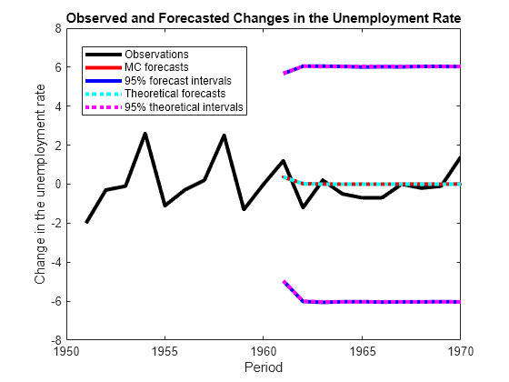
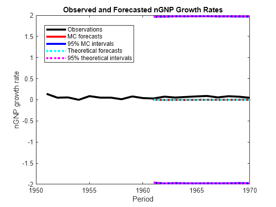
Plot the forecasted observations with their true values and the forecast intervals.
figure
h = plot(dates(end-numPeriods-9:end),[isY(end-9:end,1);oosY(:,1)],'-k',...
    dates(end-numPeriods+1:end),MCFY(end-numPeriods+1:end,1),'.-r',...
    dates(end-numPeriods+1:end),CIFY(end-numPeriods+1:end,1,1),'-b',...
    dates(end-numPeriods+1:end),CIFY(end-numPeriods+1:end,1,2),'-b',...
    dates(end-numPeriods+1:end),Y(:,1),':c',...
    dates(end-numPeriods+1:end),Lb(:,1),':m',...
    dates(end-numPeriods+1:end),Ub(:,1),':m',...
    'LineWidth',3);
xlabel('Period')
ylabel('Change in the unemployment rate')
legend(h([1,2,4:6]),{'Observations','MC forecasts',...
    '95% forecast intervals','Theoretical forecasts',...
    '95% theoretical intervals'},'Location','Best')
title('Observed and Forecasted Changes in the Unemployment Rate')

figure
h = plot(dates(end-numPeriods-9:end),[isY(end-9:end,2);oosY(:,2)],'-k',...
    dates(end-numPeriods+1:end),MCFY(end-numPeriods+1:end,2),'.-r',...
    dates(end-numPeriods+1:end),CIFY(end-numPeriods+1:end,2,1),'-b',...
    dates(end-numPeriods+1:end),CIFY(end-numPeriods+1:end,2,2),'-b',...
    dates(end-numPeriods+1:end),Y(:,2),':c',...
    dates(end-numPeriods+1:end),Lb(:,2),':m',...
    dates(end-numPeriods+1:end),Ub(:,2),':m',...
    'LineWidth',3);
xlabel('Period')
ylabel('nGNP growth rate')
legend(h([1,2,4:6]),{'Observations','MC forecasts',...
    '95% MC intervals','Theoretical forecasts','95% theoretical intervals'},...
    'Location','Best')
title('Observed and Forecasted nGNP Growth Rates')

Input Arguments
Standard state-space model, specified as anssm model
object returned by ssm or estimate. A
standard state-space model has finite initial state covariance matrix
elements. That is, Mdl cannot be a dssm model object.
If Mdl is not fully specified (that is, Mdl contains
unknown parameters), then specify values for the unknown parameters
using the 'Params' Name,Value pair
argument. Otherwise, the software throws an error.
Number of periods per path to generate variants, specified as a positive integer.
If Mdl is a time-varying model (see Decide on Model Structure), then the
length of the cell vector corresponding to the coefficient matrices must be
at least numObs.
If numObs is fewer than the number of periods
that Mdl can support, then the software only uses
the matrices in the first numObs cells of the cell
vectors corresponding to the coefficient matrices.
Data Types: double
Name-Value Arguments
Specify optional pairs of arguments as
Name1=Value1,...,NameN=ValueN, where Name is
the argument name and Value is the corresponding value.
Name-value arguments must appear after other arguments, but the order of the
pairs does not matter.
Before R2021a, use commas to separate each name and value, and enclose
Name in quotes.
Example: [Y,X] =
simulate(Mdl,numObs,'NumPaths',100)
Number of sample paths to generate variants, specified as the
comma-separated pair consisting of 'NumPaths' and
a positive integer.
Example: 'NumPaths',1000
Data Types: double
Values for unknown parameters in the state-space model, specified as the comma-separated pair consisting of 'Params' and a numeric vector.
The elements of Params correspond to the unknown parameters in the state-space model matrices A, B, C, and D, and, optionally, the initial state mean Mean0 and covariance matrix Cov0.
If you created
Mdlexplicitly (that is, by specifying the matrices without a parameter-to-matrix mapping function), then the software maps the elements ofParamstoNaNs in the state-space model matrices and initial state values. The software searches forNaNs column-wise following the orderA,B,C,D,Mean0, andCov0.If you created
Mdlimplicitly (that is, by specifying the matrices with a parameter-to-matrix mapping function), then you must set initial parameter values for the state-space model matrices, initial state values, and state types within the parameter-to-matrix mapping function.
If Mdl contains unknown parameters, then you must specify their values. Otherwise, the software ignores the value of Params.
Data Types: double
Output Arguments
Simulated observations, returned as a matrix or cell matrix of numeric vectors.
If Mdl is a time-invariant model with respect to the observations (see
Decide on Model Structure), then
Y is a
numObs-by-n-by-numPaths
array. That is, each row corresponds to a period, each column corresponds to
an observation in the model, and each page corresponds to a sample path. The
last row corresponds to the latest simulated observations.
If Mdl is a time-varying model with respect to the observations, then
Y is a
numObs-by-numPaths cell matrix of
vectors. Y{t,j} contains a vector of length
nt of simulated
observations for period t of sample path
j. The last row of Y contains the
latest set of simulated observations.
Data Types: cell | double
Simulated states, returned as a numeric matrix or cell matrix of vectors.
If Mdl is a time-invariant model with respect
to the states, then X is a numObs-by-m-by-numPaths array.
That is, each row corresponds to a period, each column corresponds
to a state in the model, and each page corresponds to a sample path.
The last row corresponds to the latest simulated states.
If Mdl is a time-varying model with respect
to the states, then X is a numObs-by-numPaths cell
matrix of vectors. X{t,j} contains a vector of
length mt of simulated states
for period t of sample path j.
The last row of X contains the latest set of simulated
states.
Simulated state disturbances, returned as a matrix or cell matrix of vectors.
If Mdl is a time-invariant model with respect
to the state disturbances, then U is a numObs-by-h-by-numPaths array.
That is, each row corresponds to a period, each column corresponds
to a state disturbance in the model, and each page corresponds to
a sample path. The last row corresponds to the latest simulated state
disturbances.
If Mdl is a time-varying model with respect
to the state disturbances, then U is a numObs-by-numPaths cell
matrix of vectors. U{t,j} contains a vector of
length ht of simulated state
disturbances for period t of sample path j.
The last row of U contains the latest set of simulated
state disturbances.
Data Types: cell | double
Simulated observation innovations, returned as a matrix or cell matrix of numeric vectors.
If Mdl is a time-invariant model with respect
to the observation innovations, then E is a numObs-by-h-by-numPaths array.
That is, each row corresponds to a period, each column corresponds
to an observation innovation in the model, and each page corresponds
to a sample path. The last row corresponds to the latest simulated
observation innovations.
If Mdl is a time-varying model with respect
to the observation innovations, then E is a numObs-by-numPaths cell
matrix of vectors. E{t,j} contains a vector of
length ht of simulated observation
innovations for period t of sample path j.
The last row of E contains the latest set of simulated
observations.
Data Types: cell | double
Tips
Simulate states from their joint conditional posterior distribution
given the responses by using simsmooth.
References
[1] Durbin J., and S. J. Koopman. Time Series Analysis by State Space Methods. 2nd ed. Oxford: Oxford University Press, 2012.
Version History
Introduced in R2014a
See Also
MATLAB Command
You clicked a link that corresponds to this MATLAB command:
Run the command by entering it in the MATLAB Command Window. Web browsers do not support MATLAB commands.
Select a Web Site
Choose a web site to get translated content where available and see local events and offers. Based on your location, we recommend that you select: .
You can also select a web site from the following list
How to Get Best Site Performance
Select the China site (in Chinese or English) for best site performance. Other MathWorks country sites are not optimized for visits from your location.
Americas
- América Latina (Español)
- Canada (English)
- United States (English)
Europe
- Belgium (English)
- Denmark (English)
- Deutschland (Deutsch)
- España (Español)
- Finland (English)
- France (Français)
- Ireland (English)
- Italia (Italiano)
- Luxembourg (English)
- Netherlands (English)
- Norway (English)
- Österreich (Deutsch)
- Portugal (English)
- Sweden (English)
- Switzerland
- United Kingdom (English)